hubtru/Siren

SIREN Scalable, Isotropic Recursive Column Multimodal Neural Architecture with Device State Recognition Use-Case

Siren

SIREN: A Scalable Isotropic Recursive Column Multimodal Neural Architecture with Device State Recognition Use-Case

Table of Contents

• Siren
  • Table of Contents
  • Introduction
    • Overview
  • Installation
  • Usage
  • SIREN Colab Demo
  • Hugging Face Space
  • Data
    • Data collection
    • Overview
    • Data structure
  • Results
    • Classification
    • Table: Sensitivity studies of number of columns on Pentostreda dataset.
    • Table: Sensitivity studies of depth of blocks on Pentostreda dataset.
    • Table: Performance comparison of various models and modalities on the Pentostreda dataset.
    • Results of MOSI and MOSEI
    • Depth-Point and Intermediate activation removal
  • Fixing the model size
    • ViT
    • MLP-Mixer:
  • Multimodal Datasets
    • The HA4M dataset:
    • Regression
  • Interpretability
    • Visualizations of the total weights of the patch embedding layers in a Siren
    • Visualization of the gradients
  • Contributing

Introduction

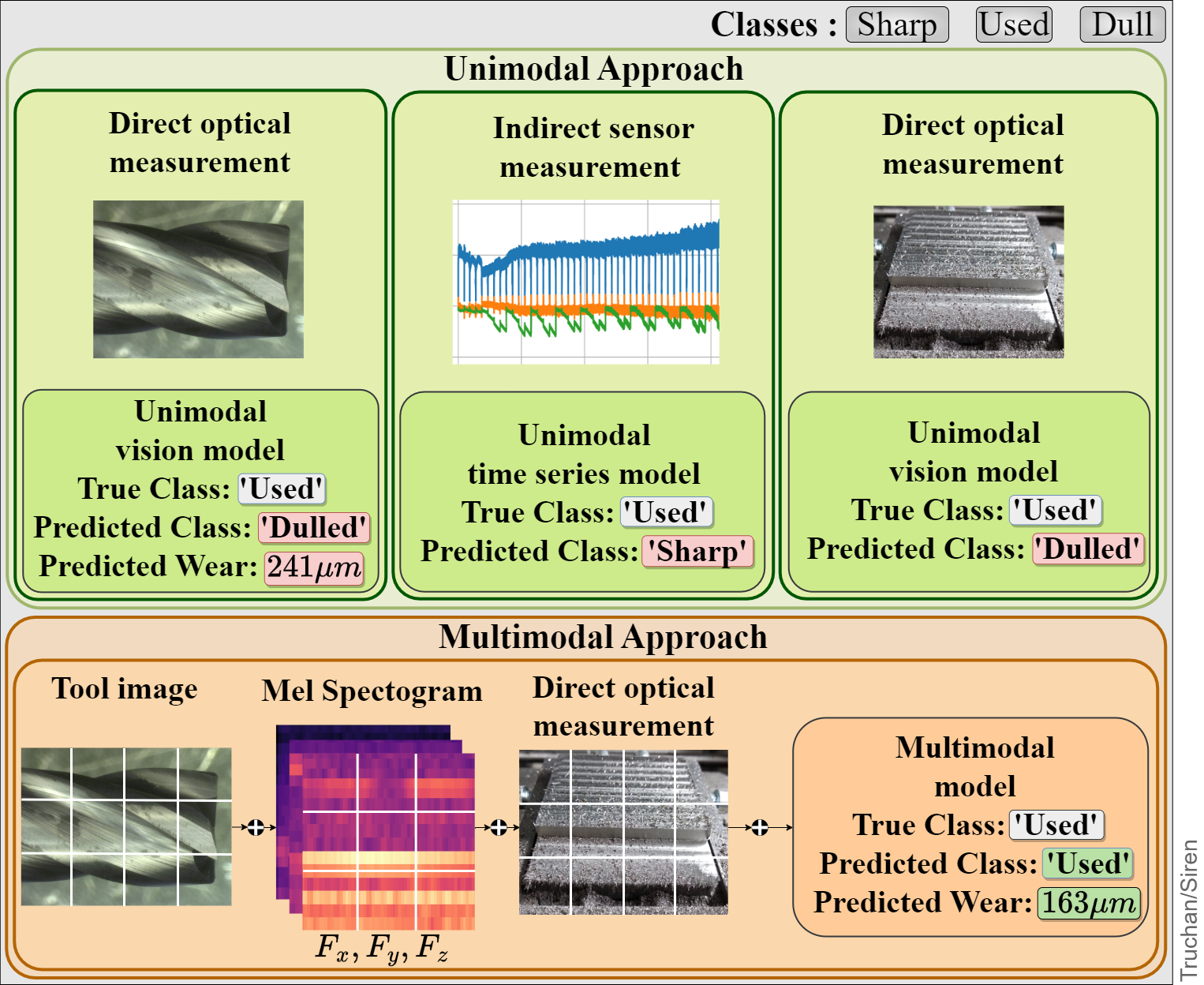
Effective monitoring of device conditions and potential damage is a critical task in various industries, including manufacturing, healthcare, and transportation. The collection of data from multiple sources poses a challenge in achieving accurate device state recognition due to its complexity and variability. To address this challenge, we propose the use of multimodal data fusion through the combination of modalities, utilizing the concentration phenomenon, to establish appropriate decision boundaries between device state regions. We introduce Siren, a novel supervised multimodal, isotropic neural architecture with patch embedding, which effectively describes device states.

Overview

Figure: A sample instance from Pentostreda that shows the importance of leveraging multimodal data for device state prediction.

The Siren uses the linearly embedded patches of the grouped signals, applies the isotropic architecture for representation retrieval, and uses TempMixer recurrent structure to map their temporal dependencies

In section Data section we present the Pentostreda : the publicly available and accessible multimodal device state recognition dataset as a new benchmark for multimodal industrial device state recognition.

Installation

Note that this work requires Python version 3.9 or later.

Install the dependencies from the requirements.txt with:

pip install -r requirements.txt

If you want to run the model on your GPU make sure to follow the installation instructions from Tensorflow.

To run .ipynb files you have to install Jupyter Notebook/JupyterLab.

In order to clone the repository to your local machine use this command

git clone https://github.com/hubtru/Siren.git

Usage

To use this project, follow these steps:

1. Download the project files to your local machine.
2. Choose the script that you want to use.

• One or multiple unimodal classification models:
  • siren_base_tool.ipynb, train and save unimodal network for tool images.
  • siren_base_spec.ipynb, train and save unimodal network for spectrogram images.
  • siren_base_chip.ipynb, train and save unimodal network for chip images.
• One or multiple multimodal classification models (requires saved unimodal .h5 models):
  • siren_base_multi_ts.ipynb, train and save multimodal network for tool and spectrogram images.
  • siren_base_multi_sc.ipynb, train and save multimodal network for spectrogram and chip images.
  • siren_base_multi_tc.ipynb, train and save multimodal network for tool and chip images.
  • siren_base_multi_tsc.ipynb, train and save multimodal network for tool, spectrogram and chip images.

---

• One or multiple unimodal regression models:
  • siren_reg_base_tool.ipynb, train and save unimodal network for tool images.
  • siren_reg_base_spec.ipynb, train and save unimodal network for spectrogram images.
  • siren_reg_base_chip.ipynb, train and save unimodal network for chip images.
• One or multiple multimodal regression models (requires saved .h5 unimodal regression models):
  • siren_reg_base_multi_ts.ipynb, train and save multimodal network for tool and spectrogram images.
  • siren_reg_base_multi_sc.ipynb, train and save multimodal network for spectrogram and chip images.
  • siren_reg_base_multi_tc.ipynb, train and save multimodal network for tool and chip images.
  • siren_reg_base_multi_tsc.ipynb, train and save multimodal network for tool, spectrogram and chip images.

3. Update the paths section in each notebook if you want they differ from the recommended setup.
4. Change the variables section if desired.
5. Run the script

Those Notebooks will run fine with the structure of the git repository. If you want to change dataset paths check the Data Structures section.

SIREN Colab Demo

The following table showcases the SIREN algorithm demonstrations for both unimodal and multimodal tasks, including their respective modalities, signals, tasks, and descriptions along with links to Colab notebooks.

Task	Type	Notebook Link	Modalities
Classification	Unimodal		Tool images
Classification	Unimodal		Spectrogram images (Fx, Fy, Fz)
Classification	Unimodal		Chip images
Classification	Multimodal		Tool images, Spectrogram images (Fx, Fy, Fz)
Classification	Multimodal		Spectrogram images (Fx, Fy, Fz), Chip images
Classification	Multimodal		Tool images, Chip images
Classification	Multimodal		Tool images, Spectrogram images (Fx, Fy, Fz), Chip images
Regression	Unimodal		Tool images
Regression	Unimodal		Spectrogram images (Fx, Fy, Fz)
Regression	Unimodal		Chip images
Regression	Multimodal		Tool images, Spectrogram images (Fx, Fy, Fz)
Regression	Multimodal		Spectrogram images (Fx, Fy, Fz), Chip images
Regression	Multimodal		Tool images, Chip images
Regression	Multimodal		Tool images, Spectrogram images (Fx, Fy, Fz), Chip images

Hugging Face Space

Check out our demonstrator on Hugging Face Spaces.

Description	Link	Task
Siren Demonstrator		Classification & Regression

Data

Pentostreda: Pento-modal Device State Recognition Dataset

Pentostreda is a five-modal data set collected from real-world milling processes over a span of seven weeks. It includes an RGB image of the milling tool, three-time series recordings of force signals, and an image that captures the metallic chips generated during the milling process. After every milling activity, an expert examined the tool's flank wear from a taken image to annotate the dataset. Depending on the observed tool wear, each instance was systematically categorized into one of three classes: new, usable, or dulled. As a result, we have created the multimodal dataset with labels, allowing us to solve the classification problem of the machine state.

• Data preview (~20 samples) is available in ./dataset
• Complete Pentostreda dataset (918MB) is available: Pentostreda (available soon)
• Complete Pentostreda.zip file (918MB) is available: Pentostreda.zip (available soon)

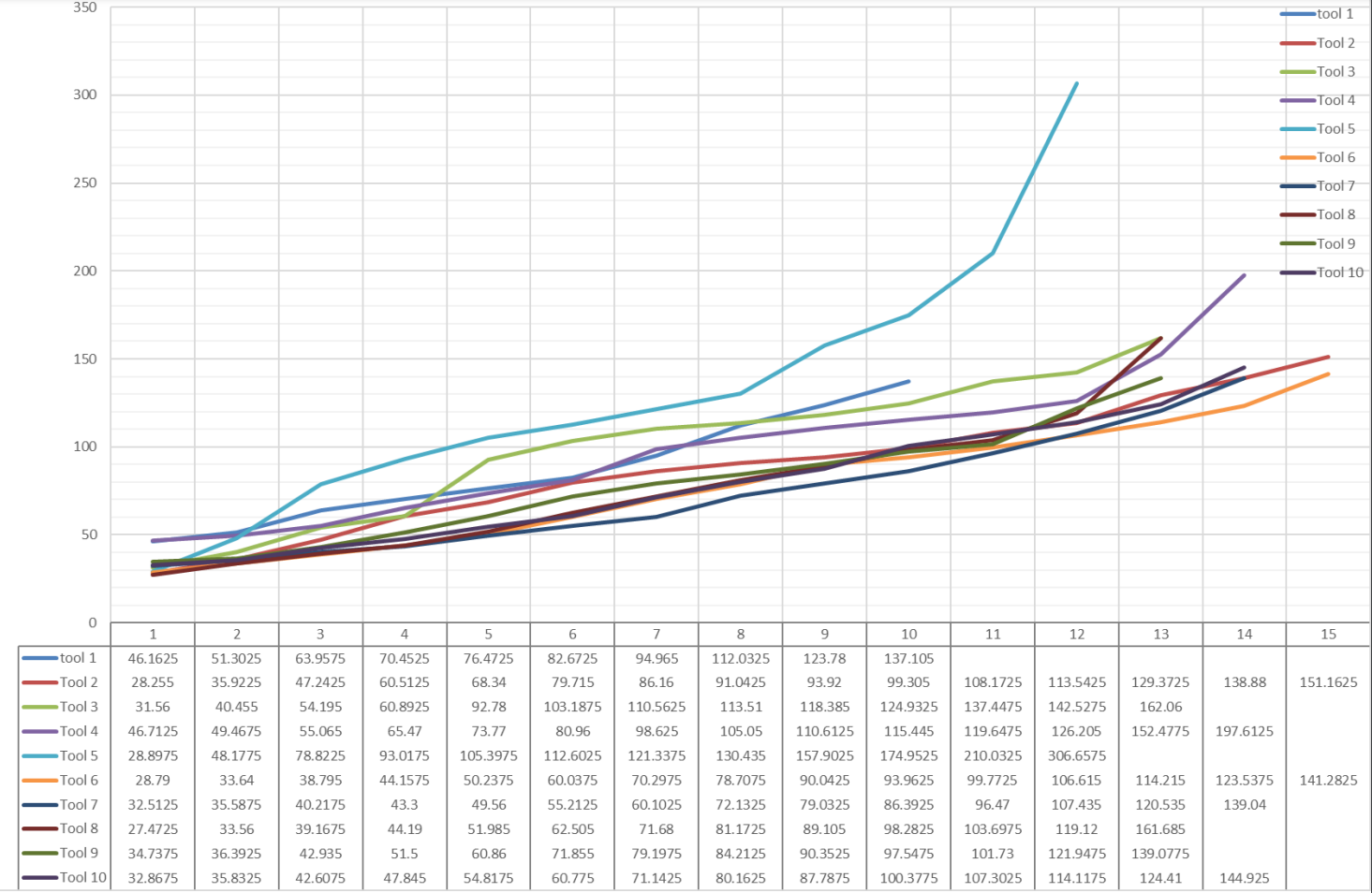
Figure: The flank tool wear measured with Keyence VHX- S15F profile measurement unit microscope for all ten tools. The values are presented in μm.

This section provides information about the data used in the project, including where it came from, how it was collected or generated, and any preprocessing or cleaning that was done.

Data collection

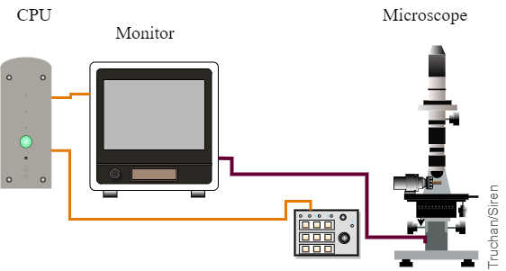
Figure: Measuring stage with the digital microscope and the industrial computer.

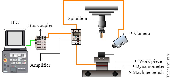
Figure: Processing stage with the signal recording diagram

Figure The forces signals depicted on Figure Signal present 30 milling phases. After each phase, a picture of the tool was taken with an industrial microscope to determine its exact wear. A strong correlation between the tool wear and the force amplitudes can be observed, with the smallest amplitudes for the sharp tool, increasing with tool wear.

Overview

The summary of the Pentostreda data-set with classes samples of Tool 1.

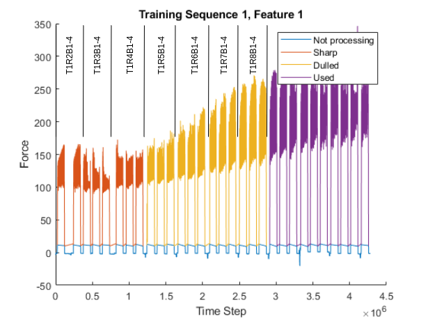
Figure: The summary of the **Pentostreda** data-set with classes samples of Tool 1. .

For more visualisation, see: Forces-Visualisation

Data structure

The folder contains the pictures of the flank wear, pictures of metal workpeace chips and the spectrograms of the forces in 3 axes (Fx, Fy, Fz).

dataset/
│
├── chip/
├── spec/x/
├── spec/y/
├── spec/z/
├── tool
│
├── labels.csv
├── labels_reg.csv
├── labels_sample.csv
└── labels_reg_sample.csv

Results

Classification

This section provides a summary of the results of the project, including any performance metrics or visualizations that were produced. It should also include a discussion of the results and their implications.

Class	Precision	Recall	F1-score
Sharp	1.00	1.00	1.00
Used	1.00	0.95	0.97
Dulled	0.92	1.00	0.96

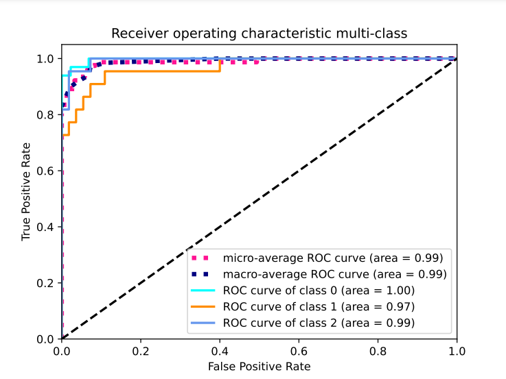
Figure: Receiver operating multi-class characteristic for SIREN hyper-band optimised multimodal (TSC: Tool, Sectrogram, Chip) model.

Table: Sensitivity studies of number of columns on Pentostreda dataset.

#Column	Flops	Size (MB)	#Params	Img/sec	Accuracy (%)
2	2711864	11	2,7M	0s 17ms/step	72.15
3	3575120	15	3,7M	0s 20ms/step	73.65
4	4438376	18	4,6M	0s 24ms/step	74.90
5	5301632	22	5,5M	0s 25ms/step	75.88
6	6164888	26	6,4M	0s 28ms/step	76.75
7	7028144	29	7,2M	0s 32ms/step	77.26
8	7891400	33	8,1M	0s 32ms/step	77.63
9	8754656	37	9,0M	0s 39ms/step	77.97
10	9617912	40	9,9M	0s 44ms/step	77.81

Table: Sensitivity studies of depth of blocks on Pentostreda dataset.

Depth	Flops	Size (MB)	#Params	Img/sec	Accuracy (%)
2	1988700	11	2.6M	16ms/step	71.63
3	2979266	15	3.6M	21ms/step	72.05
4	3631398	18	4.5M	24ms/step	74.90
5	4485996	22	5.6M	53ms/step	75.28
6	5527140	26	6.3M	70ms/step	76.43
7	6176247	29	7.3M	82ms/step	77.61
8	7038275	33	8.2M	91ms/step	77.84
9	8098056	37	8.9M	87ms/step	77.75
10	9583319	40	9.9M	110ms/step	77.53

Table: Performance comparison of various models and modalities on the Pentostreda dataset.

Model	Modality	Fusion-Type	Training	ms/img	Size(MB)	#Params	Flops	AUC	Accuracy
Meta-Transformer	t	-	1s 51ms/step	78	993.3	86.6M	85199412	0.85	57.1 (2)
Meta-Transformer	s	-	1s 51ms/step	78	993.3	86.6M	85172200	0.84	60.4 (3)
Meta-Transformer	c	-	1s 54ms/step	78	993.3	86.6M	84060374	0.85	63.9 (3)
Meta-Transformer	ts	ViT	1s 78ms/step	81	991.9	87.5M	85819362	0.83	58.5 (3)
Meta-Transformer	tc	ViT	1s 75ms/step	81	991.9	87.5M	86544254	0.85	65.3(4)
Meta-Transformer	sc	ViT	1s 73ms/step	81	991.9	87.5M	83726432	0.84	61.1 (4)
Meta-Transformer	tsc	ViT	1s 93ms/step	83	1004.5	88.3M	86367545	0.85	68.7 (4)
ViT	t	-	3s 64ms/step	36	417.4	36.4M	36375641	0.87	56.5 (3)
ViT	s	-	3s 69ms/step	44	418.2	36.4M	36473957	0.87	55.7 (4)
ViT	c	-	3s 62ms/step	35	417.4	36.5M	36375641	0.89	66.3 (2)
ViT	ts	Concat	5s 75ms/step	69	836.1	72.9M	72129427	0.88	59.2 (3)
ViT	tc	Concat	5s 62ms/step	59	835.4	72.8M	71287741	0.89	66.4 (2)
ViT	sc	Concat	5s 62ms/step	61	836.1	72.9M	73014364	0.89	67.6 (2)
ViT	tsc	Concat	8s 12ms/step	101	1252.1	109M	109111829	0.90	68.8 (3)
MLP-Mixer	t	-	1s 35ms/step	26	25.7	2.2M	2156650	0.87	57.1 (2)
MLP-Mixer	s	-	1s 36ms/step	36	30.3	2.6M	2599088	0.88	61.3 (2)
MLP-Mixer	c	-	1s 33ms/step	25	26.8	2.3M	2301206	0.87	55.4 (4)
MLP-Mixer	ts	Concat	2s 76ms/step	43	45.5	3.9M	3895658	0.89	65.7 (2)
MLP-Mixer	tc	Concat	2s 71ms/step	46	40.9	3.5M	3463465	0.88	57.6 (4)
MLP-Mixer	sc	Concat	2s 78ms/step	44	45.5	3.9M	3826508	0.89	67.2 (3)
MLP-Mixer	tsc	Concat	3s 67ms/step	53	59.5	5.1M	5086126	0.90	69.5 (2)
SIREN	t	-	2s 47ms/step	10	5.6	1.4M	1382248	0.88	58.8 (1)
SIREN	s	-	2s 53ms/step	14	7.2	1.8M	1775464	0.89	66.2 (1)
SIREN	c	-	2s 44ms/step	9	5.6	1.4M	1382248	0.90	72.5 (1)
SIREN	ts	Concat	4s 26ms/step	19	12.8	3.2M	3089991	0.90	72.9 (1)
SIREN	tc	Concat	4s 25ms/step	14	11.2	2.8M	2696775	0.90	73.7 (1)
SIREN	sc	Concat	4s 30ms/step	16	12.8	3.2M	3089991	0.90	73.3 (1)
SIREN	tsc	Concat	6s 34ms/step	23	18.1	4.5M	4438376	0.90	74.9 (1)

Results of MOSI and MOSEI

For multimodal analysis, two CMU datasets were considered:

CMU-MOSEI: 1632 samples were used for training, while the remaining 187 and 465 samples were allocated for validation and testing, respectively trained according to the predetermined protocol.

CMU-MOSI dataset: 1298 samples were categorized with a distribution of 39% positive, 35% negative, and 26% neutral.

We report the 2-class accuracy obtained through 5-fold cross-validation, following the baseline established by A. Zadeh, R. Zellers, E. Pincus, and L. Morency in their work: “MOSI: Multimodal Corpus of Sentiment Intensity and Subjectivity Analysis in Online Opinion Videos,” CoRR, vol. abs/1606.06259, 2016.

Table: Results CMU-MOSI and CMU MOSEI datasets

Model / Dataset	Mulmix	EmbraceNet	ViT	Meta-Transformer	Minape	SIREN
CMU MOSI	64.23%	72.57%	76.42%	77.89%	79.34%	83.67%
CMU MOSEI	61.48%	65.32%	74.15%	76.04%	77.21%	80.61%
Average rank	6	5	4	3	2	1

Note: Table reflects the average accuracy percentage of proposed framework compared to other methods on the CMU MOSI and CMU MOSEI multimodal benchmarks. All experiments performed on a single Nvidia GTX1080Ti 12GB GPU, results calculated over five trials.

Depth-Point and Intermediate activation removal

To copy and add as the answear The ablation results are reported for Pentostreda dataset. The base results presented in the first row. We have tested the influence of removing the intemediate activtion after the point-wise convolution [3]. We have not notices improvement, in the results. In our work we are using the improved version of activation fuction GeLU. We have conducted the ablation studies by replacing the depth-point block with fully conected bock what resulted in the decrease of the accuracies to 71.3%.

The ablation study results for the Pentostreda dataset are reported below. The baseline results are presented in the first row. We tested the impact of removing the intermediate activation function following the point-wise convolution [3]. No improvement was observed in the results. It's worth noting that in our experiments, we employed an enhanced version of the activation function, GeLU. Additionally, our ablation studies included replacing the depth-point block with a fully connected block, which led to a decrease in accuracy to 71.3%.

Table: Ablation studies on intermediate activation function

Dataset	Attention Mechanism	Cosine-Decay	Depth-Point	Intermediate Activation	Accuracy
Pentostreda	×	×	✓	✓	74.9%
Pentostreda	×	×	✓	×	74.7%
Pentostreda	×	×	×	✓	71.3%
Pentostreda	×	×	×	×	71.1%

Fixing the model size

ViT

We reduced the number of TRANSFORMER_LAYERS from 8 to 2. The outcomes of this modification are detailed in the table below.

Table: Results of the ViT with the reduced size tested on Pentostreda dataset.

Model	Modality	Fusion-Type	ms/img	Size(MB)	#Params	AUC	Accuracy
ViT	t	-	23	104.35	9.83M	0.82	38.87%
ViT	s	-	28	104.55	9.83M	0.82	38.32%
ViT	c	-	22	104.35	9.86M	0.84	45.62%
ViT	ts	Concat	44	209.03	19.68M	0.83	40.73%
ViT	tc	Concat	37	208.85	19.66M	0.84	45.68%
ViT	sc	Concat	39	209.03	19.68M	0.84	46.51%
ViT	tsc	Concat	64	313.02	29.43M	0.84	47.34%

MLP-Mixer:

We reduced the number of blocks in the MLP-Mixer from 4 to 1.

Table: Results of the MLP-Mixer with the reduced size tested on Pentostreda dataset.

Model	Modality	Fusion-Type	ms/img	Size(MB)	#Params	AUC	Accuracy
MLP-Mixer	t	-	10.4	7.453	0.682M	0.84	42.83%
MLP-Mixer	s	-	14.4	8.787	0.806M	0.84	45.97%
MLP-Mixer	c	-	10.0	7.772	0.713M	0.83	41.55%
MLP-Mixer	ts	Concat	17.2	13.195	1.209M	0.85	49.28%
MLP-Mixer	tc	Concat	18.4	11.861	1.085M	0.84	43.20%
MLP-Mixer	sc	Concat	17.6	13.195	1.209M	0.85	50.40%
MLP-Mixer	tsc	Concat	21.2	17.255	1.581M	0.86	52.13%

Multimodal Datasets

The HA4M dataset:

The HA4M dataset focuses on Multi-Modal Monitoring of an assembly task for Human Action Recognition in Manufacturing and includes six modalities: RGB images (r), Depth maps (d), IR images (i), RGB-to-Depth Alignments (g), point maps (p), and Skeleton data (s).

Table: Ablation studies. Influence of the number of modalities tested on HA4M dataset.

Model	Modality	Fusion-Type	ms/img	Size(MB)	#Params	AUC	Accuracy
SIREN	r	-	9	5.5	1.4M	0.85	47.3%
SIREN	d	-	10	6.3	1.5M	0.85	45.3%
SIREN	i	-	11	7.1	1.6M	0.84	43.3%
SIREN	g	-	12	7.9	1.7M	0.85	48.4%
SIREN	p	-	13	8.3	1.8M	0.84	44.4%
SIREN	s	-	16	8.3	1.9M	0.84	43.0%
SIREN	rd	Concat	19	15.1	2.8M	0.87	60.4%
SIREN	rdi	Concat	25	21.5	4.5M	0.89	68.5%
SIREN	rdig	Concat	34	27.8	6.7M	0.90	73.5%
SIREN	rdigp	Concat	39	35.7	8.5M	0.90	75.2%
SIREN	rdigps	Concat	48	41.3	9.7M	0.90	79.2%

Regression

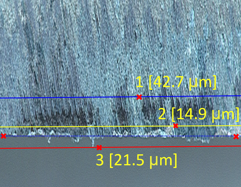
Figure: Visualisation of the base (blue-dotted), tool wear (blue), overhang (red), gaps (yellow) labels used for the regression problem.

Table: Descriptive statistics of the Pentostreda dataaset regression labels.

	Gaps	Flank	Overhang
Mean	8.20	87.86	20.95
Standard Error	0.67	2.01	0.52
Median	5.77	82.18	18.25
Mode	0	132.72	17.72
Standard Deviation	15.05	45.52	11.78
Sample Variance	226.61	2072.50	138.68
Kurtosis	48.17	4.88	2.69
Skewness	6.08	1.45	1.40
Range	154.56	324.11	76.75
Minimum	0	22.55	0
Maximum	154.56	346.66	76.75
Sum	4198.32	44985.20	10728.76
Count	512	512	512

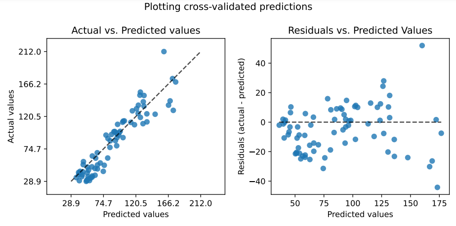
Figure: Visualisation of the actual and the residual flank wear values predicted by Siren on the Pentostreda dataset.

For more visualisation, see: interpretability/ped

Interpretability

Visualizations of the total weights of the patch embedding layers in a Siren

The total weights of the patch embedding layers in a Siren with a patch of 16 are visualized. While these layers essentially act as crude edge detectors, the industrial nature of the Mudestreda dataset prevents any discernible patterns from emerging. Interestingly, a number of filters bear a striking resemblance to noise, indicating the potential requirement for increased regularization.

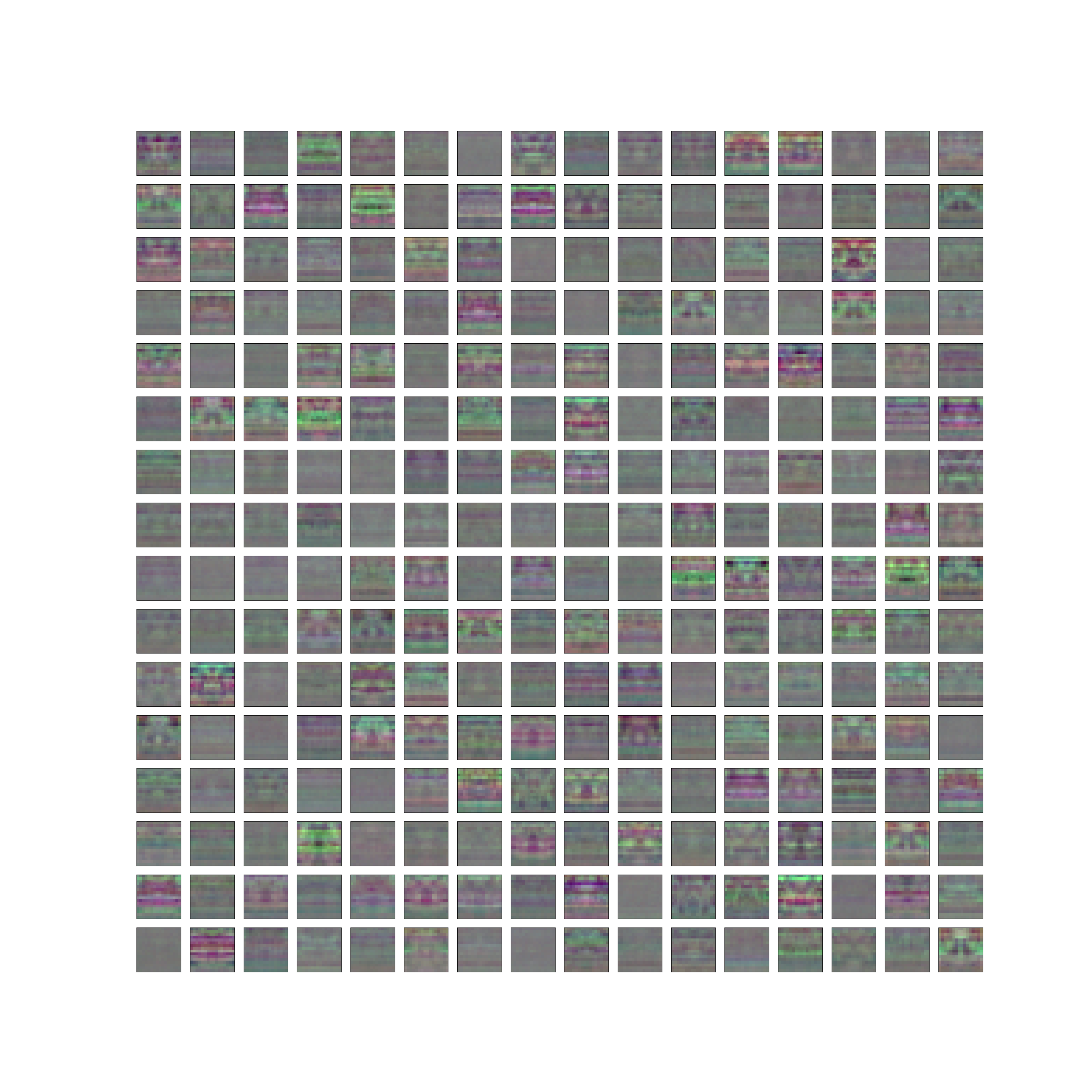
Figure: The total weights of the patch embedding layers in a SIREN with a patch of 8 for spectrogram F_x.

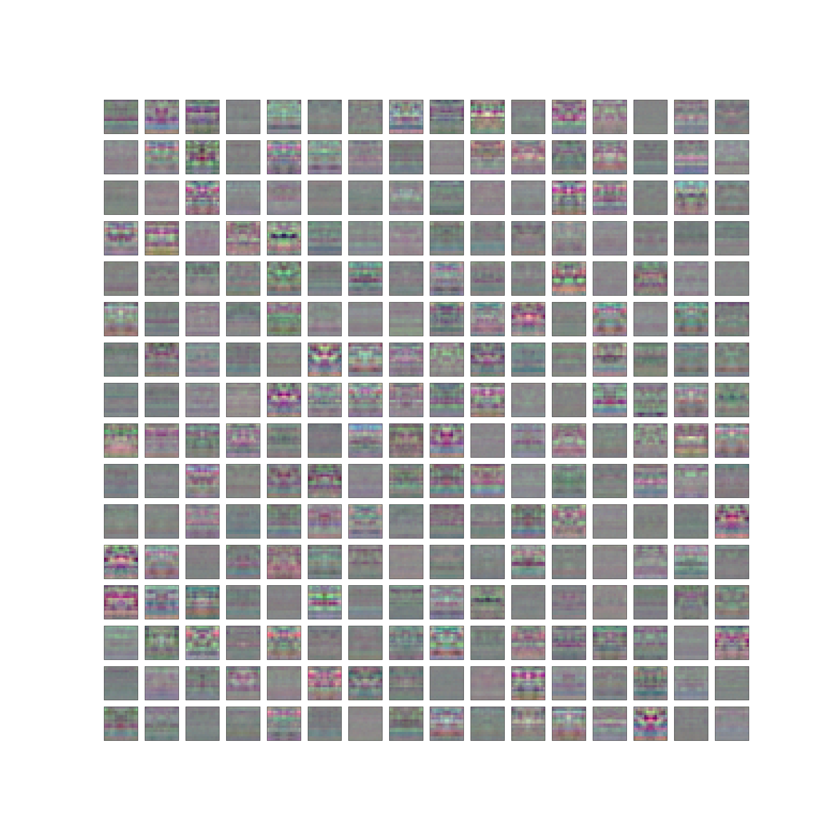
Figure: The total weights of the patch embedding layers in a SIREN with a patch of 8 for spectrogram F_y.

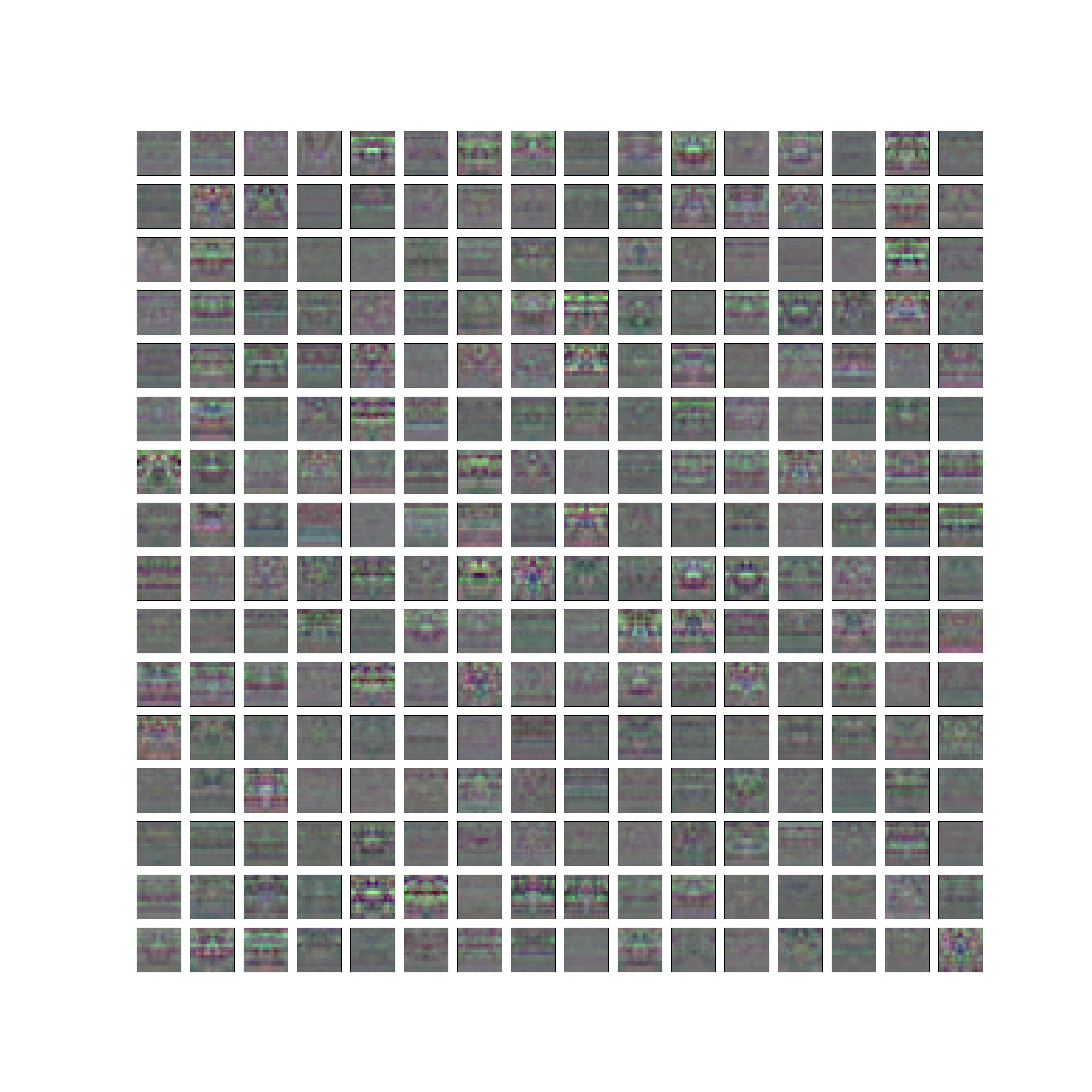
Figure: The total weights of the patch embedding layers in a SIREN with a patch of 8 for spectrogram F_z.

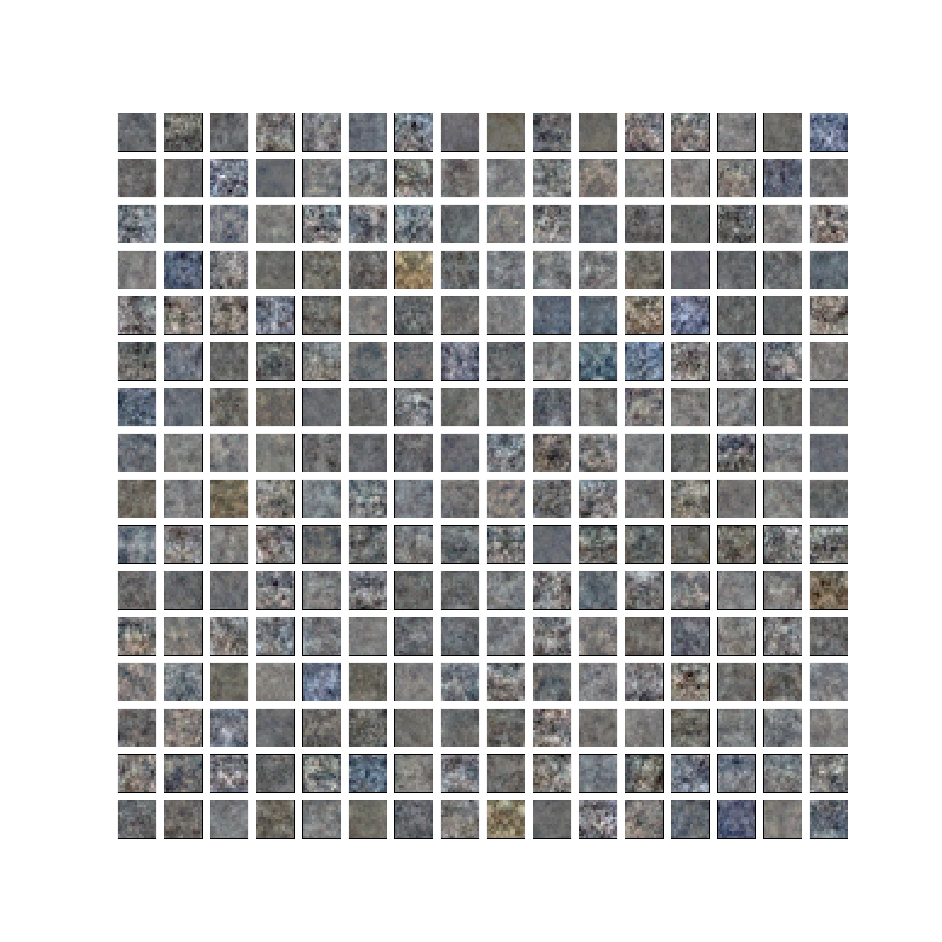
Figure: The total weights of the patch embedding layers in a SIREN with a patch of 8 for chip images.

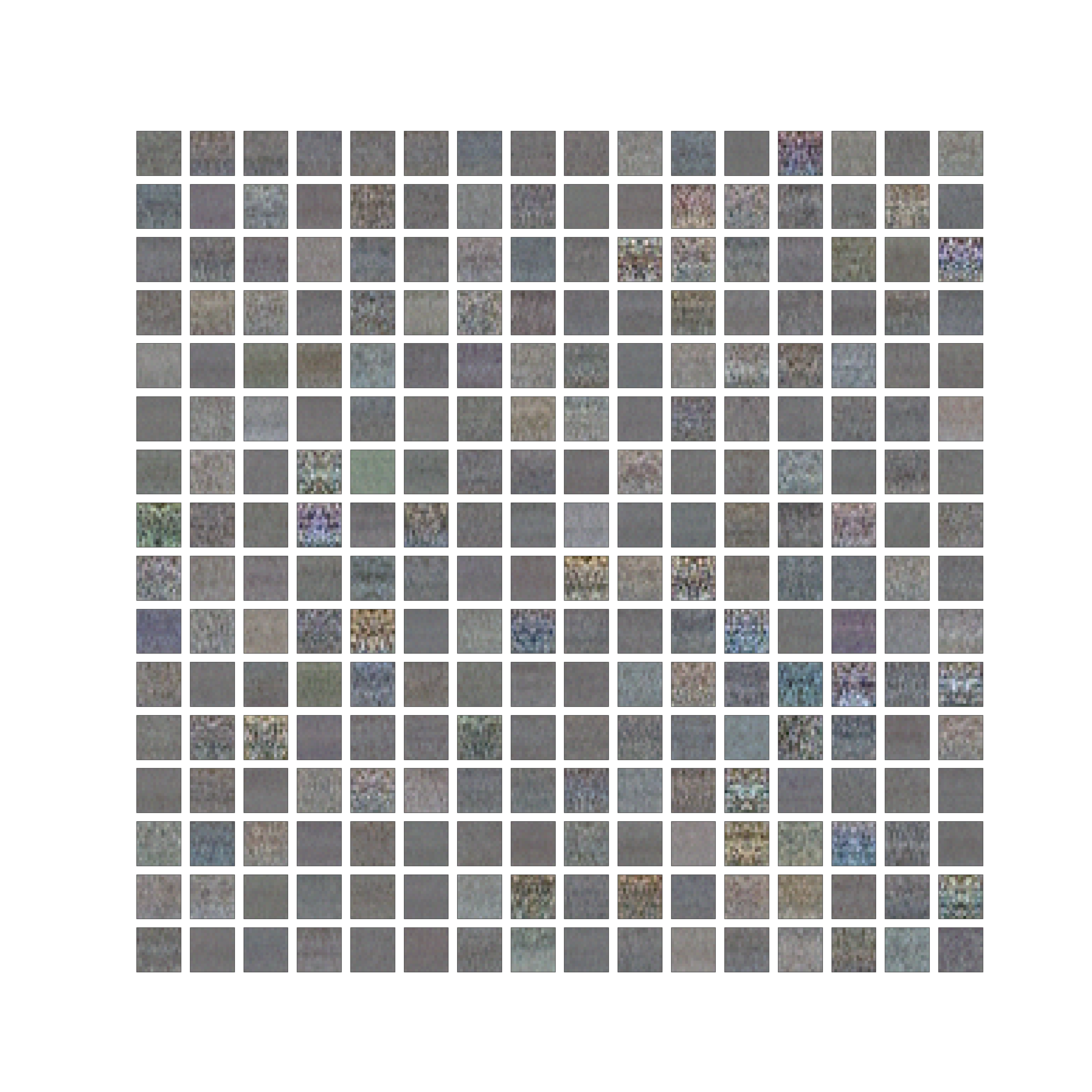
Figure: The total weights of the patch embedding layers in a SIREN with a patch of 8 for tool images.

Visualization of the gradients

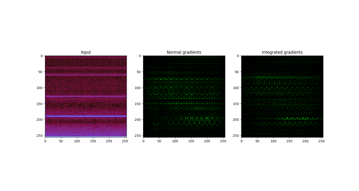
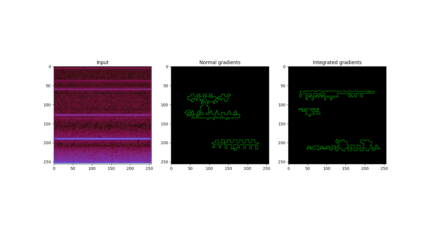
Figure: Visual comparison of normal gradient and integrated gradient on a used tool blade image. The normal gradient and integrated gradient images offer pixel-wise and area-wise importance visualization, respectively.

For more visualisation, see: interpretability

Contributing

This section provides instructions for contributing to the project, including how to report bugs, submit feature requests, or contribute code. It should also include information about the development process and any guidelines for contributing.

Pull requests are great. For major changes, please open an issue first to discuss what you would like to change.

Please make sure to update tests as appropriate.