Traffic Sign Recognition

Project Goals

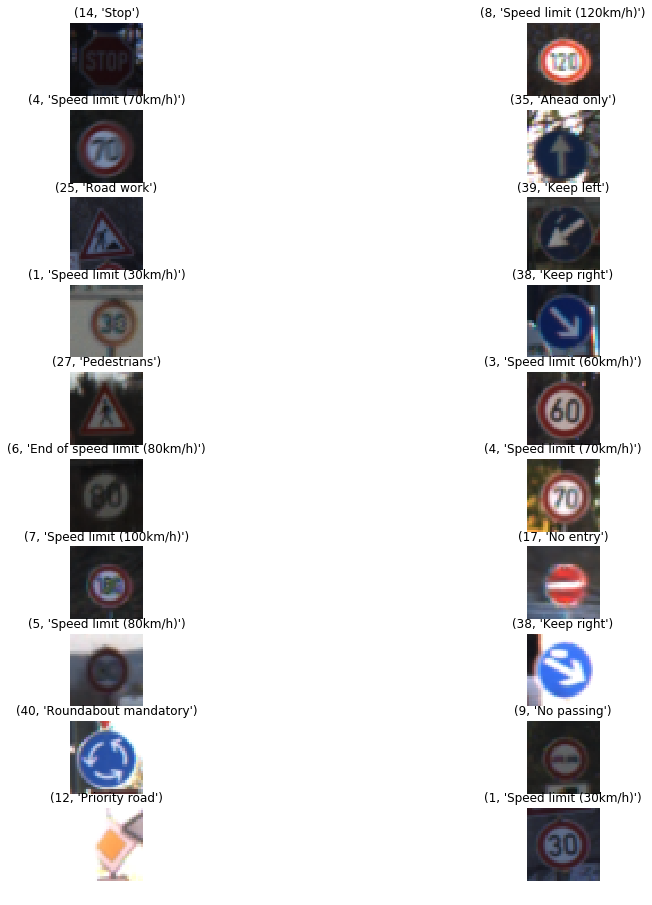
The goals of this project are the following:

Load the traffic dataset
Explore, summarize and visualize the data set
Design, train and test a CNN model architecture
Using the model to make predictions on new images downloaded from the web
Analyze the prediction(softmax) probabilities of the new images
Future improvements - point of view

1. Pipeline - Traffic Images

Pandas library is used to calculate the summary statistics of the traffic signs dataset. Training features are a 4D array (number of examples, width of an image, height of an image, color channels) of traffic sign images.

The size of the training set is: 34799,width:32, height:32, channels:3
The size of the validation set is:4410
The size of the test set is:12630
The shape of a traffic sign image is:width of 32,a height:32 and color channels:3(RBG)
The number of unique classes/labels in the data set is: 43 classes

Observations

The train data set is orderly packed.
The mapping between class ID and traffic sign name are present in a separate file called "signname.csv".
Images are smaller in size and mostly frontal view.
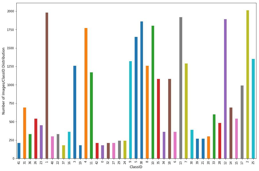
Class distribution is not even - with few outliers like Class ID 1(Speed limit (20km/h),2 (Speed limit (50km/h) and 13(Yield) followed by 12(Priority Road) and 38(Keep right).

Eyeballing Images

Class Distribution

Design and Test Model Architecture

Pre-processing the dataset(normalization, grayscale and shuffling)

The image dataset was normalized so that the data has a mean of zero and equal variance to help us to reduce the error. For image data, I used the below code to approximately normalize the dataset.

	X_train=(X_train - 128)/ 128

Image was converted to grayscale before normalization using the below code

X_train=np.sum(X_train/3, axis=3, keepdims=True)

2. Model Architecture

My final model consisted of the following layers:

Layer	Description
Layer1: Convolution	Input=32x32x1:Output=28x28x6:Filter:5x5:Stride:1x1:VALID
Layer1:RELU	Activation
Layer1:Max Pooling	Input=28x28x6:Output=14x14x6:ksize:2x2:Stride:2x2
Layer2:Convolution	Input=14x14x6:Output=10x10x16:Filter:5x5:Stride:1x1:VALID
Layer2:MaxPooling	Input=10x10x16:Output=5x5x16:ksize:2x2:Stride:2x2
Layer2:Flatten	Input=5x5x16:Output=400
Layer2:Dropout	Keep Probability:0.5
Layer3:FullyConnected	Input=400:Output=120
Layer3:RELU	Activation
Layer3:Dropout	Keep Probability:0.5
Layer4:FullyConnected	Input=120:Output=84
Layer4:RELU	Activation
Layer4:Dropout	Keep Probability:0.5
Layer5:FullyConnected	Input=84:Output=43

3. Model Training

Model training was iterative as the validation accuracy was below 80% despite choosing a well known architecture created by Pierre Sermanet and Yann LeCun (http://yann.lecun.com/exdb/publis/pdf/sermanet-ijcnn-11.pdf). I changed the hyper parameters to make sure that the model is generalized for testing. All adjustments on model architecture was due to overfitting i.e. a high accuracy on the training set but low accuracy on the validation set. Addition of a dropout layer with a slower learning rate helped to generalize the model. The final hyper parameters are:

_epochs =150
_batchSize=128
_dropout= 0.5 #forcing few weights to play dump
_learningRate = 0.0006 #slower rate 0.001 or 0.002 was resulting in less than 80%

Final Results

Validation Accuracy = 0.972
Test Accuracy with Model 2.0 = 0.952
Test Accuracy with Model 1.0 = 0.944

Model Tracking

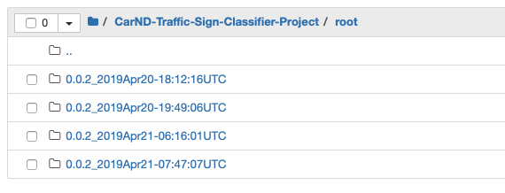
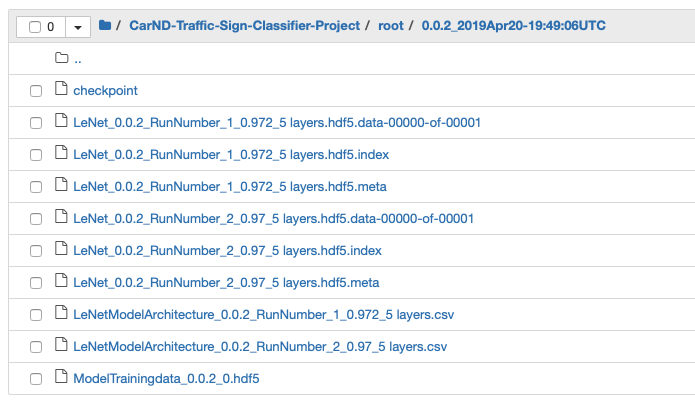
I implemented a tracking nomenclature since it was extremely difficult to keep track of model architecture, hyperpram and date & time. This approach helped me quickly organize my model training effort and save time. Please see below:

Details of the model can be tracked:

4. Testing model generalizability

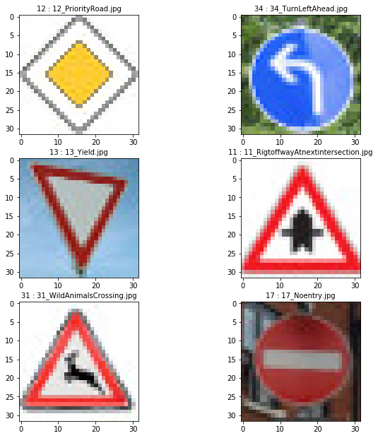
This was done to check model accuracy if subjected to a new image from the internet. The model performed well as the images were preprocessed to meet the input needs i.e. 32x32x1 with good amount of luminosity.

The model was able to identify the images correctly. Web sample test accuracy = 1.000

Please see the prediction outputs:

5. Top five softmax probabilities for the predictions

For each of the new images, I used the model's softmax probabilities function to show the certainty of the model's predictions.

_topCounter=5 #top five softmax probabilities
_softmaxLogits = tf.nn.softmax(logits)
_top_k=tf.nn.top_k(_softmaxLogits,_topCounter)

with tf.Session() as sess:
    _saver = tf.train.import_meta_graph('./root/0.0.2_2019Apr21-07:47:07UTC/LeNet_0.0.2_RunNumber_2_0.974_5 layers.hdf5.meta')
    _saver.restore(sess, tf.train.latest_checkpoint('./root/0.0.2_2019Apr21-07:47:07UTC/'))
    _softmaxProbabilities = sess.run(_top_k, feed_dict={x: X_test_web, keep_prob: 1.0})
    print(_softmaxProbabilities)

Output of tf.nn.top_k(softmax probabilities)

Actual ClassID 12==>Predicted Class ID: 12(100%), 40(2.18e-11%), 13(2.41e-15),  9(3.15e-18), 42(2.9e-18)
Actual ClassID 34==>Predicted Class ID: 34(9.99e-01), 38(2.85e-4), 13(1.1e-8), 35(9.05e-11),  9(8.07e-11)
Actual ClassID 13==>Predicted Class ID: 13(1.0e+00), 12(1.49e-31), 35(1.37e-34), 15(1.38e-36),0(0.0+00)
Actual ClassID 11==>Predicted Class ID: 11(9.99e-01), 30(3.34e-06), 27(2.53e-10), 21(1.22e-11),25(9.18e-13)
Actual ClassID 31==>Predicted Class ID: 31(9.99e-01), 19(4.10e-06),23(2.33e-07),21(2.19e-07),29(1.23e-08)
Actual ClassID 17==>Predicted Class ID: 17(9.99e-01), 14(4.78e-05),38(8.44e-07),12(6.33e-08),0(8.25e-09)

6. Future Improvements

The main difficulty will be to create label data to make a generalized model capable of handling real world scenarios like diffrent view angles, distortion, damaged signs, hidden portions etc. It would be nice to test and extend other well known models like Inception V3, VGG 16/19, ResNet50. It would be also interesting to create complementary models to train and cross-train on good label data and intentionally mislabeled data.

Challenge

The main challenge for an image recognition model is creating a vast amount of label data.

iPhoring/TrafficSignRecognition