Organizer's note: this project won the industry choice award in iQuHACK 2020.
We:
- Perform VQE on a massive Schwinger model Hamiltonian and
- Explore its applications to MC simulations on classical computers.
In (1), we reproduce the results of 1801.03897. In (2), we are ultimately interested in transition matrix elements such as
The Schwinger model is a (1+1)D theory of quantum electrodynamics (QED). It describes fermions as a two-component spinor field , with mass
, coupled via charge
to an electromagnetic field
in infinite continuum space, with the Lagrangian given by
To simulate the system, we need to put in on a finite lattice. Generally, one has to be careful with latticizing the theory with spinor degrees of freedom to correctly retrieve the Dirac equation in the continuum limit; an approach that works, that was used in recent quantum-computer simulations and that we will also employ is a Kogut-Susskind staggered lattice formulation. On a staggered lattice, the two spinor components are put on neighboring sites. Finally, we use a Jordan-Wigner transformation to map the fermionic degrees of freedom to bosonic ones. The final form of the Hamiltonian suitable for simulations on quantum computers is given by
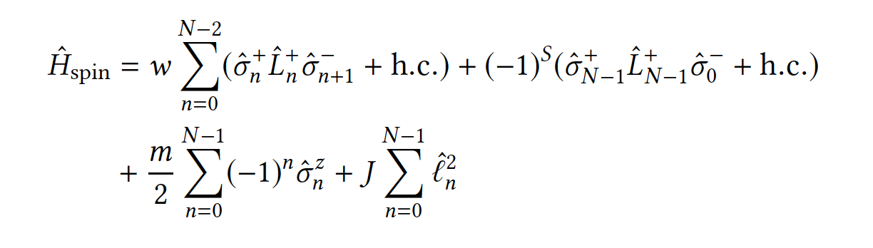
where is the total spin of the spin chain, and the number of spatial sites on the lattice,
, is even. The coupling constants are given by
and
.
- For our simulations (see Mathematica notebooks), we set
, which fixes
.
- We then specify dimensionless parameters
and
.
- The latter fixes
.
- We set
and
.
-
-
- At these values, the predictions should match. Note that in Martin's paper, the Hamiltonian (and eigenenergies) are measured in units of
; to match our measurements with those reported by Martin, multiply their predictions by the value of
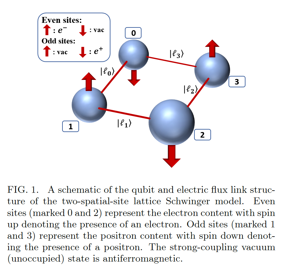
- We use a Kogut-Susskind formulation at a finite volume of two spatial sites. To reduce qubit requirements, we consider only a small, physically relevant section of the Hilbert space (and hence, a smaller Hamiltonian).
- We achieve the reduction by considering only translationally invariant states (zero three-momentum) of definite parity. This block-diagonalizes a zero-momentum Hamiltonian into two H_+ and H_-, corresponding to sectors of even and odd parity.
- Finally, we truncate on the allowed values of electric field flux on the links of the lattice, discarding high-energy states.
- We then perform two separate VQE simulations on truncated H_+ and H_-.
- We have a Mathematica script that performs all the Hilbert space restrictions mentioned above.
- With this code, we exactly diagonalize the truncated H_+ and H_- at the same numerical values of all parameters.
- Further, we derive the variational ansatz that is capable of approximating the ground state exactly: a change-of-basis matrix that rotates a Hamiltonian from the computational basis into its diagonal form.
- Although we find a circuit that yields the required rotation matrix, we find that it would be too costly too implement. Therefore, we opt for a cheaper circuit that can approximate the exact ansatz numerically.
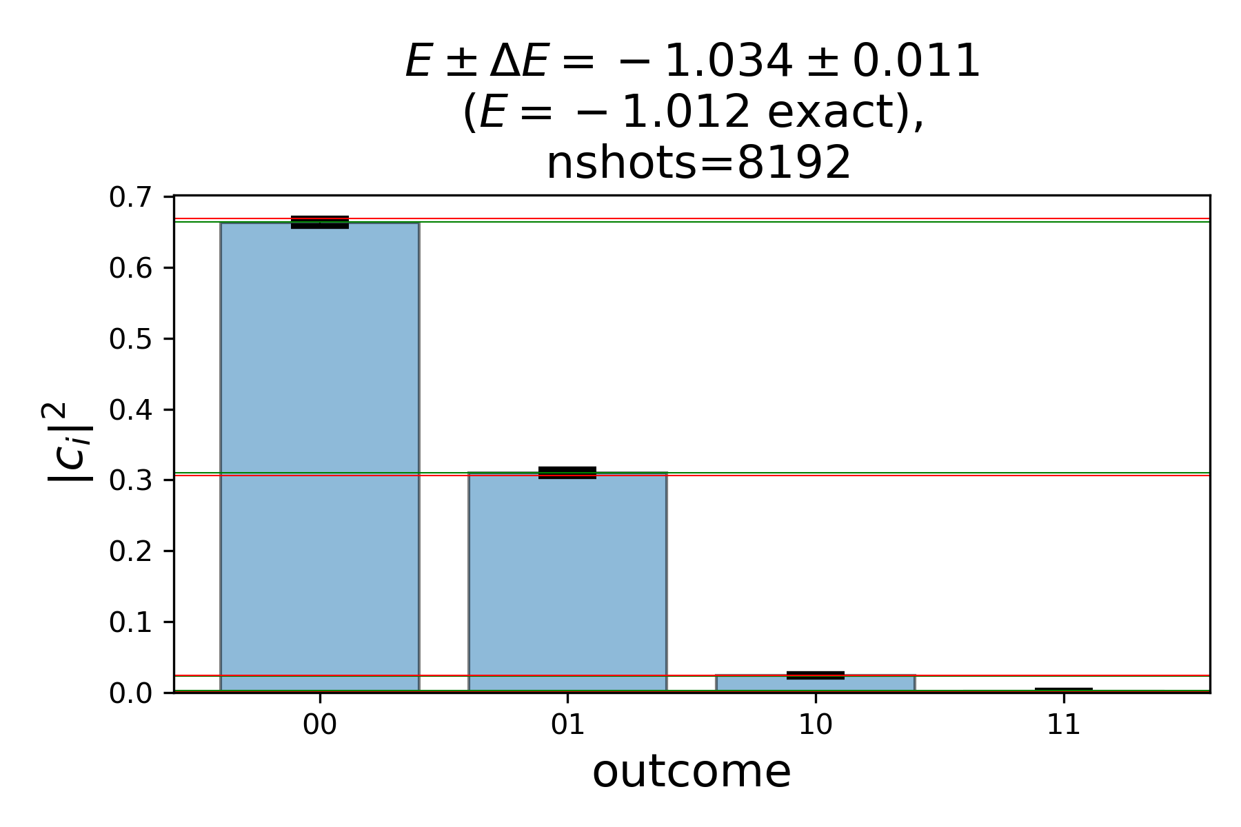
- For VQE ran on a simulator, we find excellent agreement with our exact solution.
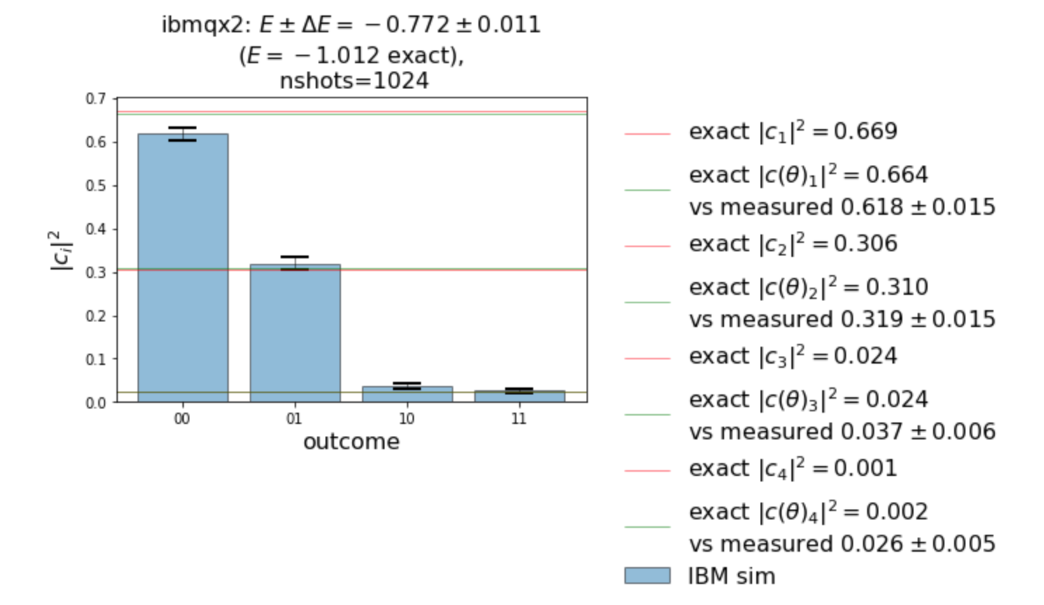
- For VQE ran on a quantum device (imbq_yorktown), we find fair agreement with the results reported by 1801.03897.
- We found the VQE workflow to be very slow when run on quantum devices through IBM's queuing system, with each iteration queued separately and sequentially.
- Some of the inefficiency may come from the SPSA optimizer, whose default parameters are not fine-tuned for the system in question. From studying the convergence properties of the optimizer, both on a simulator and the quantum device, we think that convergence can be achieved significantly faster by tuning SPSA's annealing parameters.
- For our runs on real quantum devices, we expect sizeable improvement from:
- Employing error-mitigation strategies
- Addressing readout errors
- Further optimizing a circuit with a transpiler.
- Exploring other IBM quantum devices, and potentially combining results from devices with different error profiles.
- Due to the inefficiency of the workflow on real quantum devices, we find the ability to add noise models to the simulators extremely helpful to prototyping solutions. We have already started working on that.
- With our Mathematica script that performs the Hilbert space reduction, we find the numerical form of the transition operators in the computational basis of the quantum computer.
- To measure the off-diagonal matrix elements --- transition amplitudes between two variational states --- we devise a strategy that requires a preparation of superpositions of 2 variational states.
- We have prototyped circuits to perform this preparation that all work as expected on the simulators, but are currently prohibitively expensive in the presence of noise on real quantum devices. We are currently looking for other possible implementations of this idea:
- One direction involves a variational approach. But we have not found a cost function whose ground state would be the superposition of two variational states.
- Another direction is to find a circuit that utilizes known variational parameters and circuits for preparing the two variational states separately. This direction would benefit from a previous question we encountered when designing an efficient variational layer: given an exact and computationally expensive circut, how does one find its cheaper approximation? Or, if you wish, how can one approximate a given quantum channel with a fixed number of resources?
- savage.ipynb is the original Jupyter notebook used to play with VQE workflow. It uses Qiskit minimally, so that all the different parts are explicit and verbose. This may be helpful when trying to understand what Qiskit does behind the scenes.
- VQE.ipynb is the main notebook for a VQE simulations. Still in development. Ultimately, this needs be a Python module/package. But the current Jupyter-notebook form is convenient for playing around with the code and learning Qiskit's functionality. Different parts of the VQE workflow have smaller notebooks. They're not required to run the main one, but are convenient if you want to look at an isolated element of the simulation.
- Superposition.ipynb is the Jupyter with a circuit for producing a superposition of the variational states (ground state and first excited state)
Mathematica code (exact diagonalization)
- savage.nb is the main notebook that performs projection onto zero-momentum sector, truncation, and splits the resulting Hilbert space into even and odd parity sectors. It diagonalizes the corresponding Hamiltonians, expresses the eigenstates in the computational basis of the QC simulation. Interpolating operators are constructed and exact effective mass curves are computed.
- variational_layer.nb is a notebook to play with the form of the variational layer in the QC simulation as an explicit unitary.
- operators.nb is a notebook where the numerical matrix form of the interpolators is computed in the (concatenated) QC computational basis of even and odd parity sectors.