Numerical Monte Carlo solution to the system of stochastic differential equations of population dynamics

Goals and objectives

The aim of this project was to apply Itô's stochastic differential equations (SDEs) theory for the particular problem from population biology and to compare a stochastic competition model model with a deterministic one. In order to gain better understanding of this theory, several problems were covered:

Stochastic process modelling.
Itô's stochastic integral modelling and approximate calculation of its expectations.
Obtaining numerical solutions to stochastic differential equation (SDE) using Monte-Carlo simulation.

Methods

Itô's lemma

Let F be a function F(t, X(t)) and X be a stochastic process such that

$dX = \mu_t dt + \sigma dW$

then (assuming the necessary assumptions) function F satisfies the following SDE:

$dF = \left(\frac{\partial F}{\partial t} + \mu \frac{\partial F}{\partial x} + \frac{1}{2}\sigma^2 \frac{\partial^2 F}{\partial x^2}\right)dt + \sigma \frac{\partial F}{\partial x} dW$

Itô's lemma allows us to find closed-form solution to some SDEs and exactly calculate some stochastic integrals.

Monte Carlo simulation

Monte Carlo simulation is a computational algorithm that relies on random sampling to obtain numerical result. Pseude-random numbers obtained from Numpy generator were used to simulate randomness.

System requirements

Most of the project (except population dynamics modelling) was implemented using laptop with the following resources: Intel(R) Core(TM) i5-8300H CPU @ 2.30Ghz, 8GB RAM, Windows 10

Python and libraries:

Python 3.8.5
Numpy 1.19.1
Scipy 1.5.0
Matplotlib 3.3.1
Seaborn 0.11.0

Population dynamics modelling was implemented in Google colab (with free access plan). Language and libraries versions are the following:

Python 3.6.9
Numpy 1.19.4
Scipy 1.4.1
Matplotlib 3.2.2
Seaborn 0.11.0
Numba 0.48.0

Results and examples

There's a small library for stochastic modelling and calculus: StoCalc.py. It is built atop of Scipy and Numpy and provides functions for modelling stochastic processes and integrals, calculation of stochastic integral expectations, and solving SDEs.

1. Weiner process

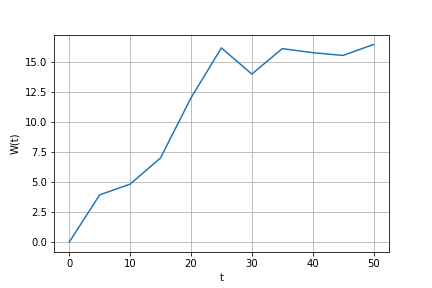
Obtain one Weiner process sample path on interval [0, 50] with step = 5:

import matplotlib.pyplot as plt
import numpy as np
from StoCalc import weiner_process

np.random.seed(0)

time1, proc1 = weiner_process(t0=0, T=T, m=1, N=11)
plt.plot(time1, proc1)

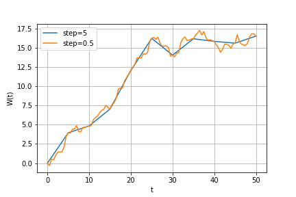
Add more points to this trajectory (so that step would be 0.5):

from StoCalc import brownian_bridge

new_points = np.arange(0, T, 0.5)
time2, proc2 = brownian_bridge(np.array([time1, proc1[0]]), new_points)

plt.plot(time1, proc1[0], label='step=5')
plt.plot(time2, proc2, label='step=0.5')

2. Itô's stochastic integrals

Consider the following Itô's integral:

$I(f) = \int_0^1f(t, W(t))dW(t) = \int_0^1t \cdot e^{W(t)}dW(t)$

Calculate first 3 moments, i.e. E(I(f)), E(I²(f)), E(I³(f)), with step=0.01 and different sample size:

from StoCalc import ito_int_expect
np.random.seed(0)

def f(t, Wt):
    return t * np.exp(Wt)

sample_sizes = (10, 100, 10000)
ks = (1, 2, 3)  # moment orders
for size in sample_sizes:
    tmp = [size]
    for k in ks:
        tmp.append(ito_int_expect(f, 0, 1, k, m=size))
    print(*tmp, sep='\t')  
    
# output:
# 10     0.124  1.163  0.106
# 100    0.116  0.729  0.859
# 10000  0.009  1.291  5.864

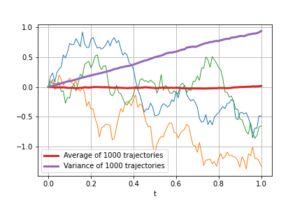
Generate 1000 samples, plot the first 3 of them, average and variance of trajectories:

from StoCalc import ito_int_paths
np.random.seed(0)

time, paths = ito_int_paths(f, 0, 1, step=0.01, m=1000)

for p in paths[:3]:
    plt.plot(time, p, linewidth=1)
plt.plot(time, paths.mean(axis=0), linewidth=3, label='Average of 1000 trajectories')
plt.plot(time, paths.var(ddof=1, axis=0), linewidth=3, label='Variance of 1000 trajectories')

3. Stochastic differential equations

Consider the following SDE:

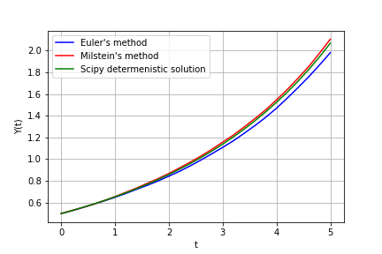
$\begin{cases} dY(t) = f\cdot dt + g\cdot dW(t)=\left( \frac{1}{4} Y(t) + \frac{1}{32}Y^2(t) \right)dt + \frac{1}{4}Y(t)dW(t),\ \\ Y(0) =\frac{1}{2} \end{cases}$

Obtain 1000 solutions using Euler's and Milstein's method and compare average of 1000 solutions for both methods with Scipy-provided solver for a corresponing determenistic ODE:

from StoCalc import sde
np.random.seed(0)

def dyE(y, dt, dW):
    f = 1/4 * y + 1/32 * y**2
    g = 1/4 * y
    return (f, g) 

def dyM(y, dt, dW):
    f = 1/4 * y + 1/32 * y**2
    g = 1/4 * y
    dgdy = 1/4   # need to provide additional derivative for Milstein's method
    return f, g, dgdy

y0 = 1/2
step = 1/5  # step size is large to see the difference between methods
t = (0, 5)

time, pathsE = sde(dyE, y0, t, step, method='euler')  # Euler's method
time, pathsM = sde(dyM, y0, t, step, method='milstein')  # Milstein's method

# determenistic equation
from scipy.integrate import odeint

def det_dydt(y, t):
    return 1/4 * y + 1/32 * y**2

sol = odeint(det_dydt, y0, time)

plt.plot(time, pathsE.mean(axis=0), color='blue', label="Euler's method")
plt.plot(time, pathsM.mean(axis=0), color='red', label="Milstein's method")
plt.plot(time, sol, color='green', label='Scipy determenistic solution')

See examples for more.

4. Population dynamics applications

Finally, Itô's theory was applied to the population biology system of two populations that are in competition (see Modelling.ipynb for the exact problem formulation).

The stochastic model was compared to the corresponding determenistic model, and the solutions did not exactly match. Most noticable is the fact that the mean population size estimation is much different from the determenistic result, because in the stochastic model there are 2 possible end states and both populations have a probability to go extinct. The stochastic model was used to estimate extinction probabilities, extinction time and conditional probability density for sizes of both populations. Mean conditional extincton time for the second population is also less then extinction time from the determenistic model because of the chance to survive:

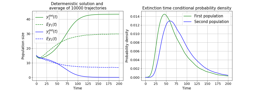
See Modelling.ipynb for conditional probability densities and modelling source code.

References

Allen, Edward. (2007). Modeling with Itô Stochastic Differential Equations. 22. 10.1007/978-1-4020-5953-7.
Choongbum Lee, Peter Kempthorne, Vasily Strela, Jake Xia. 18.S096 Topics in Mathematics with Applications in Finance. Fall 2013. Massachusetts Institute of Technology: MIT OpenCourseWare, https://ocw.mit.edu/. License: Creative Commons BY-NC-SA.

iam28th/SDE