A collection of functions to simplify and speed up High Energy Physics research with Python.
To install the package to your home directory with pip, run
pip install --user git+https://github.com/ibab/missing_hepA class for working with four momenta is provided.
To use it, pass values or arrays to the FourMomentum constructor:
from missing_hep import FourMomentum

P = FourMomentum(10, 1, 2, 3)
print(P.mass())
# 9.2736184954957039

from math import sqrt
print(sqrt(P * P))
# 9.2736184954957039
FourMomentum is also designed to work with arrays of numbers (for example, columns from a pandas DataFrame):
import numpy as np
X = np.random.uniform(0, 100, size=10)

P = FourMomentum(X, 0, 0, X)

print(P.mass())
# array([ 0., 0., 0., 0., 0., 0., 0., 0., 0., 0.])In High Energy Physics, histograms are often displayed as a collection of data points, one for each bin. This allows one to easily compare the data to an underlying probability model.
It can be debated if it is correct to attach error bars to the individual bin contents as opposed to the underlying model, as we want to know if our expectation could fluctuate to become the data and not vice versa. But this is a convention widely used by the HEP community, and thus a way to use this style of plotting in Python is often necessary.
A simple way to create these kinds of plots is missing from other Python packages like matplotlib.
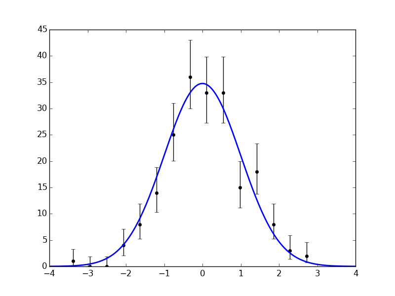
The histpoints function is designed to produce these plots conventiently, like in the following example:
from missing_hep import histpoints
import matplotlib.pyplot as plt
import numpy as np
import scipy.stats as stats

data = np.random.normal(0, 1, 200)
x, y, norm = histpoints(data)

xs = np.linspace(-4, 4, 200)
plt.plot(xs, norm * stats.norm.pdf(xs, 0, 1), 'b-', lw=2)

plt.savefig('histpoints.png')
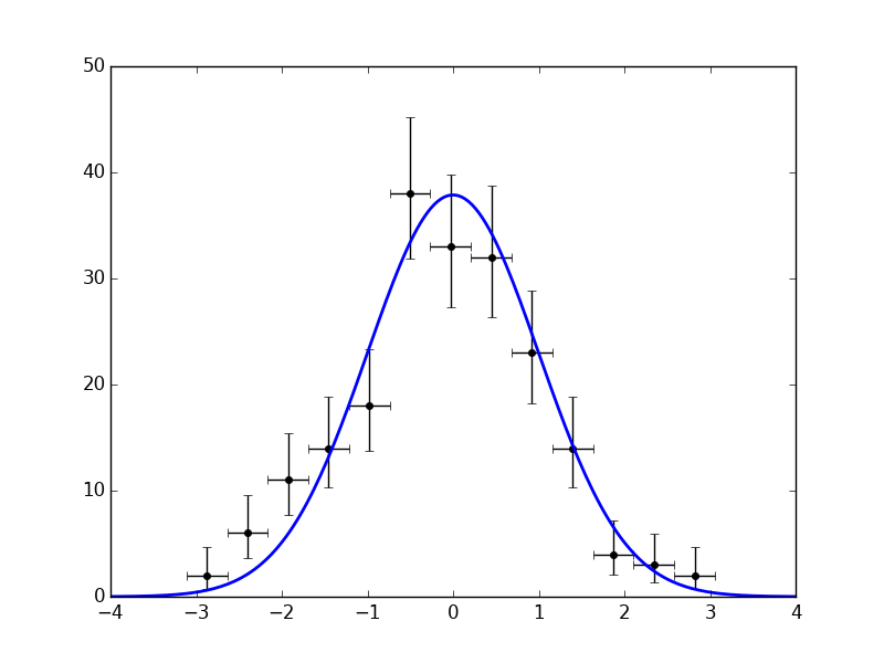
Or, displaying horizontal error bars to mark the bin width:
histpoints(data, xerr='binwidth')By default, the number of bins is chosen automatically via the Freedman-Diaconis rule.
Notice also that the vertical error bars in this example are asymmetric, as opposed to the symmetric sqrt(N) error bars often seen in HEP publications.
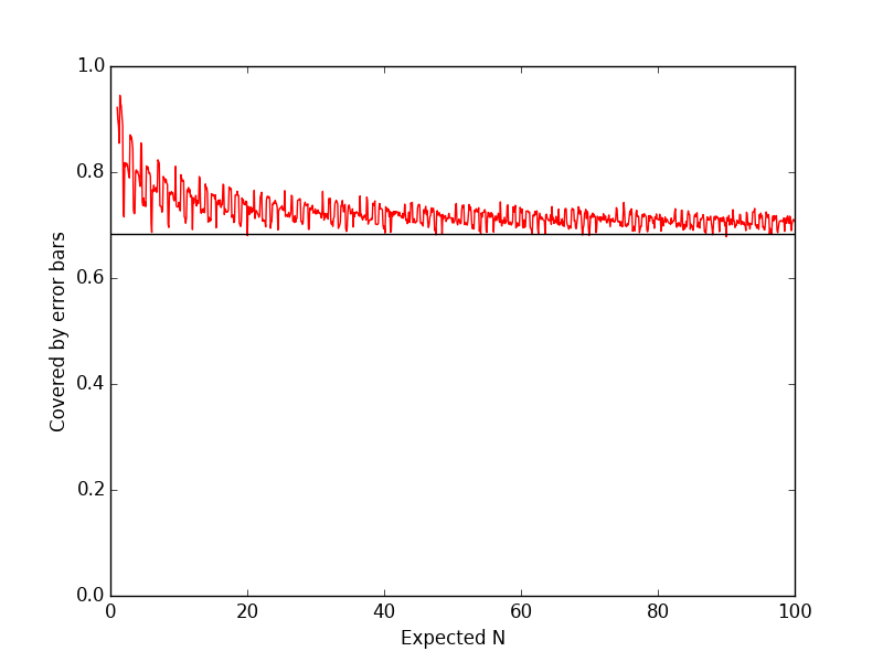
By default, histpoints uses the gamma distribution to calculate asymmetric error bars.
The frequentist coverage properties of this approach can be seen from the following demonstration:
import numpy as np
from scipy.stats import poisson, gamma
import matplotlib.pyplot as plt

def err(N, confidence=0.6827):
    alpha = 1 - confidence
    upper = np.zeros(len(N))
    lower = np.zeros(len(N))
    lower = gamma.ppf(alpha / 2, N)
    lower[N==0] = 0
    upper = gamma.ppf(1 - alpha / 2, N + 1)
    return N - lower, upper - N

cov = []

Ns = np.linspace(1, 100, 1000)

for N in Ns:
    data = poisson.rvs(N, size=10000)
    lower, upper = err(data)
    inside = sum((data - lower <= N) & (N <= data + upper))
    cov.append(inside / len(data))

plt.plot(Ns, cov, 'r-')
plt.axhline(0.6827, color='k')
plt.ylim(0, 1)
plt.ylabel('Covered by error bars')
plt.xlabel('Expected N')
plt.savefig('coverage.png')

