![]()
Playground to explore Monte Carlo generators properties.
Inspired by Fooled by Randomness.
List of experiments, consult the section below for a detailed overview:
- Coin toss with / without ruin.
- Pi estimation
If you have go already installed the easiest thing to do is to grab the package via go get:
go get -u github.com/igor-kupczynski/monte-carlo-explorationThis installs the binaries, but also puts the resources in your $GOPATH so you can run the included experiments, e.g.
monte-carlo-exploration --conf $GOPATH/src/github.com/igor-kupczynski/monte-carlo-exploration/examples/cointoss.tomlAlternatively, if you don't have go or don't want to install the package you can grad the latest binaries publish by github actions.
-
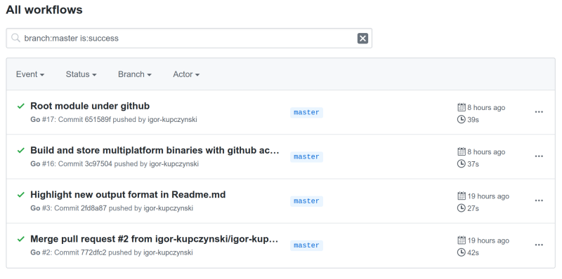
Select the latest build from the list.
This would be Root module under github in the screenshot below:
-
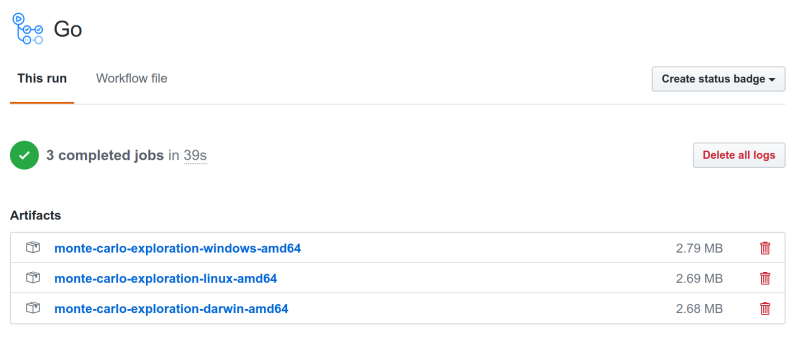
Download the package for your operating system -- windows, linux, or macos (this would be under darwin):
-
Extract the distribution.
E.g. from the command line:
$ unzip monte-carlo-exploration-linux-amd64.zip -d monte-carlo-exploration
Archive:  monte-carlo-exploration-linux-amd64.zip
  creating: monte-carlo-exploration/examples/
 inflating: monte-carlo-exploration/LICENSE
 inflating: monte-carlo-exploration/monte-carlo-exploration
 inflating: monte-carlo-exploration/README.md
 inflating: monte-carlo-exploration/examples/cointoss-no-ruin.toml
 inflating: monte-carlo-exploration/examples/cointoss.toml
You may also need to make the binary executable on linux and macos:
$ chmod +x monte-carlo-exploration/monte-carlo-exploration
-
Run the experiments:
$ cd monte-carlo-exploration
$ ./monte-carlo-exploration --conf examples/cointoss.toml
# Run simulation examples/cointoss.toml
## Simulating 1000000 executions of 100 round coin toss with starting capital of $10

ruined: 31.963400% (319634 / 1000000)
Less capital: 48.864000% (488640 / 1000000)
More capital: 44.266900% (442669 / 1000000)
p01 $0
p05 $0
p10 $0
p25 $0
p50 $10
p75 $16
p90 $22
p95 $26
p99 $34


-
Checkout this repo :)
-
Get dependencies:
$ go get -v -t -d ./...
-
Build:
$ go build -v . -
Run tests:
$ go test -v ./...
Simulate multiple rounds of coin tossing. Heads we get $1, tails we pay $1. We have $10 starting capital, but drawing it down to $0 means ruin, and we can't continue the game.
# Run simulation examples/cointoss.toml
## Simulating 1000000 executions of 100 round coin toss with starting capital of $10

Dataset [len=1000000, baseline=10]
* Avg=10.013292	Min=0	Max62
* % of items below=48.804000%	at=6.875000%	above=44.321000% baseline
* Percentiles:
	- p01%: 0	baseline diff: -100.000000%
	- p05%: 0	baseline diff: -100.000000%
	- p10%: 0	baseline diff: -100.000000%
	- p25%: 0	baseline diff: -100.000000%
	- p50%: 10	baseline diff: 0.000000%
	- p75%: 16	baseline diff: 60.000000%
	- p90%: 22	baseline diff: 120.000000%
	- p95%: 26	baseline diff: 160.000000%
	- p99%: 34	baseline diff: 240.000000%
* % ruined: 31.987300%
I wound't play that -- 30%+ chance of ruin. We end up with more capital only <45% of the time, and with less >48%.
Let's ignore ruin for now. $100 and 100 rounds. We can go to ruin only in the last round.
$ ./monte-carlo-exploration --conf examples/cointoss-no-ruin.toml
# Run simulation examples/cointoss-no-ruin.toml
## Simulating 1000000 executions of 100 round coin toss with starting capital of $100

Dataset [len=1000000, baseline=100]
* Avg=99.993434	Min=48	Max148
* % of items below=46.088100%	at=7.908000%	above=46.003900% baseline
* Percentiles:
	- p01%: 76	baseline diff: -24.000000%
	- p05%: 84	baseline diff: -16.000000%
	- p10%: 88	baseline diff: -12.000000%
	- p25%: 94	baseline diff: -6.000000%
	- p50%: 100	baseline diff: 0.000000%
	- p75%: 106	baseline diff: 6.000000%
	- p90%: 112	baseline diff: 12.000000%
	- p95%: 116	baseline diff: 16.000000%
	- p99%: 124	baseline diff: 24.000000%
* % ruined: 0.000000%
Good sport, seems a fair game! Only 1% of the time we lose more than $24, and only 1% we earn more than $24.
This is a different example to show that Monte Carlo is a general purpose method.
We have a circle:

We know that the area of the circle is proportional to its radius squared times Pi. We would like to estimate the value of Pi.
The circle is inscribed in the square. Its radius is 0.5 * square's side.
A = Pi * r^2
Pi = 4 * A / d^2
We can estimate the circle area by throwing darts into the circle image. We select (x, y) pairs by random and record if the pair is in the circle or outside of it.
Each simulation consists of 10000 games. We start with throwing 1000 darts and then increase this by the factor of 10, until we hit 1 million. The image is 1024 x 1024 so at this point it's hard to get a better result unless we switch to a larger image.
# Run simulation examples/pi_1k.toml
## Pi estimation: 10000 executions of 1000 dart throws to examples/circle.png

Dataset [len=10000, baseline=3141592654]
* Avg=3142455600.000000	Min=2940000000	Max3328000000
* % of items below=49.700000%	at=0.000000%	above=50.300000% baseline
* Percentiles:
	- p01%: 3020000000	baseline diff: -3.870414%
	- p05%: 3056000000	baseline diff: -2.724499%
	- p10%: 3076000000	baseline diff: -2.087879%
	- p25%: 3108000000	baseline diff: -1.069287%
	- p50%: 3144000000	baseline diff: 0.076628%
	- p75%: 3180000000	baseline diff: 1.222544%
	- p90%: 3212000000	baseline diff: 2.241135%
	- p95%: 3228000000	baseline diff: 2.750431%
	- p99%: 3264000000	baseline diff: 3.896347%
We cheat a little because we know what the Pi really is. This is what we record as a baseline.
To avoid float point arithmetics by scale by billion and do the calculations with int64.
We can see that 1000 darts is not enough. While the median of 10000 runs is only 0.07% off, if we take the [p5, p95] percentiles we are over/under shot by almost 3, i.e. [-2.724499%, 2.750431%].
Let's see if we can improve with more darts throws.
# Run simulation examples/pi_10k.toml
## Pi estimation: 10000 executions of 10000 dart throws to examples/circle.png

Dataset [len=10000, baseline=3141592654]
* Avg=3141925320.000000	Min=3080800000	Max3205600000
* % of items below=48.250000%	at=0.000000%	above=51.750000% baseline
* Percentiles:
	- p01%: 3102800000	baseline diff: -1.234809%
	- p05%: 3114800000	baseline diff: -0.852837%
	- p10%: 3120400000	baseline diff: -0.674583%
	- p25%: 3130800000	baseline diff: -0.343541%
	- p50%: 3142000000	baseline diff: 0.012966%
	- p75%: 3153200000	baseline diff: 0.369473%
	- p90%: 3162800000	baseline diff: 0.675051%
	- p95%: 3168800000	baseline diff: 0.866037%
- p99%: 3180000000 baseline diff: 1.222544%# Run simulation examples/pi_100k.toml
## Pi estimation: 10000 executions of 100000 dart throws to examples/circle.png
Dataset [len=10000, baseline=3141592654]
* Avg=3141721236.000000 Min=3122160000 Max3159320000
* % of items below=48.650000% at=0.000000% above=51.350000% baseline
* Percentiles:
- p01%: 3129520000 baseline diff: -0.384285%
- p05%: 3133120000 baseline diff: -0.269693%
- p10%: 3135000000 baseline diff: -0.209851%
- p25%: 3138200000 baseline diff: -0.107992%
- p50%: 3141760000 baseline diff: 0.005327%
- p75%: 3145240000 baseline diff: 0.116099%
- p90%: 3148360000 baseline diff: 0.215411%
- p95%: 3150240000 baseline diff: 0.275254%
- p99%: 3154160000 baseline diff: 0.400031%# Run simulation examples/pi_1m.toml
## Pi estimation: 10000 executions of 1000000 dart throws to examples/circle.png
Dataset [len=10000, baseline=3141592654]
* Avg=3141744172.000000 Min=3132896000 Max3147716000
* % of items below=46.440000% at=0.000000% above=53.560000% baseline
* Percentiles:
- p01%: 3137928000 baseline diff: -0.116650%
- p05%: 3139024000 baseline diff: -0.081763%
- p10%: 3139628000 baseline diff: -0.062537%
- p25%: 3140604000 baseline diff: -0.031470%
- p50%: 3141740000 baseline diff: 0.004690%
- p75%: 3142872000 baseline diff: 0.040723%
- p90%: 3143876000 baseline diff: 0.072681%
- p95%: 3144468000 baseline diff: 0.091525%
- p99%: 3145512000 baseline diff: 0.124757%With more darts we can see that we are getting closer to the result, and we can also be more confident in the result -- looking at the p10 and p90 percentiles.
| Number of darts | p5 error | p95 error |
|---|---|---|
| 1k | -2.724499% | 2.750431% |
| 10k | -0.852837% | 0.866037% |
| 100k | -0.269693% | 0.275254% |
| 1m | -0.081763% | 0.091525% |
I suspect with the 1m we are at a point of diminishing returns. The result is not too impressive -- within ~0.1% error from the true value 90% of the time -- it is too far to practical. We could easily improve this by taking a larger image and increasing the number of dart throws. We could improve it by a few orders of magnitude with this technique.
The circle is generated with GIMP and the image is not black-and-white. It is a bit fuzzy and grayscale at the edges of the circle. Initially, I've considered 50% gray to be black (so within the circle), but I've noticed we are underestimating PI. E.g. with 100k darts we've had:
# Run simulation examples/pi_100k.toml
## Pi estimation: 10000 executions of 100000 dart throws to examples/circle.png

Dataset [len=10000, baseline=3141592654]
* Avg=3137947812.000000	Min=3119040000	Max3157720000
* % of items below=75.760000%	at=0.000000%	above=24.240000% baseline
...
75% of the estimations were below the true value. Then I've switched to consider anything non-white as black. Looks like we are much more balanced now.
- Stock price behavior. (what's the distribution? how to get it's params?)
- Options pricing.