The GoldenCheetahOpenData R package provides methods for querying
the GoldenCheetah OpenData project database <doi:
10.17605/OSF.IO/6HFPZ>, downloading workout data from it and managing
local workout databases. Methods are also provided for the organization
of the workout data into trackeRdata objects for further data analysis
and modelling in R using the infrastructure provided by the trackeR
R package
https://CRAN.R-project.org/package=trackeR.
You can install the released version of GoldenCheetahOpenData from CRAN with:
install.packages("GoldenCheetahOpenData")
The development version can be installed directly from GitHub with:
# install.packages("devtools")
devtools::install_github("ikosmidis/GoldenCheetahOpenData")
GoldenCheetahOpenData implements a simple query-download-read workflow, that allows users to gradually build and maintain a local repository with workouts from the GoldenCheetah OpenData project.
The first step in the GoldenCheetahOpenData R package workflow is to
query the mirrors of the GoldenCheetah OpenData project for the
available IDs. This is done with a call to get_athelte_ids(), which
will create a gcod_db object.
library("GoldenCheetahOpenData")
ids <- get_athlete_ids()
class(ids)
#> [1] "gcod_db" "list"
gcod_db objects have two perspectives: a remote perspective describing
the state of the GoldenCheetah OpenData project’s database, and a local
describing the state of any local database (more on this later).
gcod_db objects that are produced by get_athlete_ids() have no
records in their local perspective because none have been downloaded.
print(ids, txtplot = TRUE)
#> Remote perspective
#> Mirror: S3
#> Number of athlete IDs: 6576
#> File sizes: min = 301 bytes | max = 251.8 Mb | total = 107.2 Gb
#> Last modified: between 2018-11-17 10:20:38 and 2020-05-27 07:46:13
#> Athlete ID records modified per year quarter:
#>      +--+-----------+----------+----------+----------+----------+----------+---+
#>      |                                                          =              |
#>   25 +  =                                                       =              +
#>      |  =                                                       =              |
#> A    |  =                                                       =              |
#> t 20 +  =                                                       =          =   +
#> h    |  =                                                       =          =   |
#> l    |  =                                                       =          =   |
#> e 15 +  =                                                       =          =   +
#> t    |  =                                                       =          =   |
#> e 10 +  =           =                                           =          =   +
#> s    |  =           =                                           =          =   |
#>      |  =           =          =                                =          =   |
#> %  5 +  =           =          =          =                     =          =   +
#>      |  =           =          =          =          =          =          =   |
#>      |  =           =          =          =          =          =          =   |
#>    0 +  =           =          =          =          =          =          =   +
#>      +--+-----------+----------+----------+----------+----------+----------+---+
#>         1           2          3          4          5          6          7
#> Legend:
#> 1=2018-10-01, 2=2019-01-01, 3=2019-04-01, 4=2019-07-01, 5=2019-10-01, 6=2020-01-
#> 01, 7=2020-04-01
#>
#> Local perspective
#> Number of athlete IDs: 0
The output above also gives us a quick snapshot of GoldenCheetah OpenData project’s database. It currently has
format(total_size(ids), unit = "auto")
#> [1] "107.2 Gb"
worth of compressed workout sessions for
n_ids(ids, perspective = "remote")
#> [1] 6576
athletes. And it keeps growing!
gcod_db objects can directly be passed into the download_workouts()
function for getting the workouts for the athlete IDs in the remote
perspective or at least a few of them. Below we only get the workouts
for those athletes whose IDs contain b7-9 (as a big fan of the Star
Trek Voyager series,
this choice made sense to me!).
ids_b79 <- download_workouts(ids,
                             pattern = "b7-9",
                             local_dir = "~/Downloads/GCOD-db/",
                             verbose = TRUE)
#> Downloading 6f0380b7-92d0-4c19-a56d-85ac3bf472a6.zip (5.9 Mb) ... Done.
#> Downloading a3ccd92b-87f0-422d-adb7-91ab3e6021aa.zip (21.7 Mb) ... Done.
#> Downloading af3ab0e9-fc82-43b7-9d5b-60d496b77d70.zip (2.7 Mb) ... Done.
#> Downloading e104e895-9ecc-40b7-9e62-c1c8823ae0d8.zip (9.7 Mb) ... Done.
After the above code chunk was run, download_workouts() downloaded the
requested workout data on my disk and placed them in the directory
“~/Downloads/GCOD-db/”
dir("~/Downloads/GCOD-db")
#> [1] "6f0380b7-92d0-4c19-a56d-85ac3bf472a6.zip"
#> [2] "a3ccd92b-87f0-422d-adb7-91ab3e6021aa.zip"
#> [3] "af3ab0e9-fc82-43b7-9d5b-60d496b77d70.zip"
#> [4] "e104e895-9ecc-40b7-9e62-c1c8823ae0d8.zip"
The result from download_workouts() is a new gcod_db object, which
has updated the local and remote perspectives of the original gcod_db
object
ids_b79
#> Remote perspective
#> Mirror: S3
#> Number of athlete IDs: 4
#> File sizes: min = 2.7 Mb | max = 21.7 Mb | total = 39.9 Mb
#> Last modified: between 2019-08-05 07:33:44 and 2020-05-08 20:10:44
#>
#> Local perspective
#> Number of athlete IDs: 4
#> File sizes: min = 2.7 Mb | max = 21.7 Mb | total = 39.9 Mb
#> Last modified: between 2020-05-27 18:41:50 and 2020-05-27 18:42:23
You may save your gcod_db files, but this is not really necessary.
They can be reconstructed using the rebuild_bd() method, which reads
the local workout database and makes appropriate queries to the
GoldenCheetah OpenData project’s mirrors:
ids_dir <- rebuild_db("~/Downloads/GCOD-db")
ids_dir
#> Remote perspective
#> Mirror: S3
#> Number of athlete IDs: 4
#> File sizes: min = 2.7 Mb | max = 21.7 Mb | total = 39.9 Mb
#> Last modified: between 2019-08-05 07:33:44 and 2020-05-08 20:10:44
#>
#> Local perspective
#> Number of athlete IDs: 4
#> File sizes: min = 2.7 Mb | max = 21.7 Mb | total = 39.9 Mb
#> Last modified: between 2020-05-27 18:41:50 and 2020-05-27 18:42:23
ids_b79
#> Remote perspective
#> Mirror: S3
#> Number of athlete IDs: 4
#> File sizes: min = 2.7 Mb | max = 21.7 Mb | total = 39.9 Mb
#> Last modified: between 2019-08-05 07:33:44 and 2020-05-08 20:10:44
#>
#> Local perspective
#> Number of athlete IDs: 4
#> File sizes: min = 2.7 Mb | max = 21.7 Mb | total = 39.9 Mb
#> Last modified: between 2020-05-27 18:41:50 and 2020-05-27 18:42:23
athlete_id(ids_dir, perspective = "local")
#> [1] "6f0380b7-92d0-4c19-a56d-85ac3bf472a6"
#> [2] "a3ccd92b-87f0-422d-adb7-91ab3e6021aa"
#> [3] "af3ab0e9-fc82-43b7-9d5b-60d496b77d70"
#> [4] "e104e895-9ecc-40b7-9e62-c1c8823ae0d8"
athlete_id(ids_b79, perspective = "local")
#> [1] "6f0380b7-92d0-4c19-a56d-85ac3bf472a6"
#> [2] "a3ccd92b-87f0-422d-adb7-91ab3e6021aa"
#> [3] "af3ab0e9-fc82-43b7-9d5b-60d496b77d70"
#> [4] "e104e895-9ecc-40b7-9e62-c1c8823ae0d8"
athlete_id(ids_dir, perspective = "remote")
#> [1] "e104e895-9ecc-40b7-9e62-c1c8823ae0d8"
#> [2] "a3ccd92b-87f0-422d-adb7-91ab3e6021aa"
#> [3] "6f0380b7-92d0-4c19-a56d-85ac3bf472a6"
#> [4] "af3ab0e9-fc82-43b7-9d5b-60d496b77d70"
athlete_id(ids_b79, perspective = "remote")
#> [1] "6f0380b7-92d0-4c19-a56d-85ac3bf472a6"
#> [2] "a3ccd92b-87f0-422d-adb7-91ab3e6021aa"
#> [3] "af3ab0e9-fc82-43b7-9d5b-60d496b77d70"
#> [4] "e104e895-9ecc-40b7-9e62-c1c8823ae0d8"
Caution! A careless call to download_workouts() can easily instruct R
to start downloading all workouts from the GoldenCheetah OpenData
project, which is rarely what you want. Instead, I recommend downloading
only a few at a time. This can be done in various ways, including using
the prefix argument of get_athlete_ids(), the pattern argument of
download_workouts() (as above) or — a bit more advanced — by directly
subsetting the gcod_db object
ids_sub <- subset(ids, subset = grepl("b7-9", athlete_id(ids)), perspective = "remote")
athlete_id(ids_sub)
#> [1] "6f0380b7-92d0-4c19-a56d-85ac3bf472a6"
#> [2] "a3ccd92b-87f0-422d-adb7-91ab3e6021aa"
#> [3] "af3ab0e9-fc82-43b7-9d5b-60d496b77d70"
#> [4] "e104e895-9ecc-40b7-9e62-c1c8823ae0d8"
In this way, whenever you rebuild the gcod_db object form the local
database you are getting access to all the workout files you have ever
downloaded.
Reading workouts involves: extracting the workout archives for each
athlete ID, reading all the .csv files in the extracted directories,
wrangling the information in them (e.g. inferring the workout
timestamps, carrying out data quality checks, imputation, etc), and
organizing the resulting data into objects that can be used for further
analyses. The read_workouts() method can do all the above from a
unified interface. For example (and this takes a while):
b79 <- read_workouts(ids_b79)
By default, read_workouts(): - does not overwrite existing directories
with extracted workouts (which can be bypassed by setting
overwrite = TRUE) - deletes the extracted directories after everything
has been read (which can be bypassed by setting clean_db = FALSE) -
writes the processed trackeRdata objects (see ?saveRDS) in the same
directory as the workout archives, using the convention
<athlete_id>.rds.
b79 is now a list of trackeRdata objects, and trackeR can be
used for exploration.
library("trackeR")
## Reading was not possible for athlete ID (see `warnings`)
which(is.na(b79))
#> a3ccd92b-87f0-422d-adb7-91ab3e6021aa
#>                                    2
## so we remove them
b79 <- b79[!is.na(b79)]
## number of workout sessions per athlete ID
sapply(b79, nsessions)
#> 6f0380b7-92d0-4c19-a56d-85ac3bf472a6 af3ab0e9-fc82-43b7-9d5b-60d496b77d70
#>                                   84                                   47
#> e104e895-9ecc-40b7-9e62-c1c8823ae0d8
#>                                  274
## total duration per athlete ID in hours
sapply(b79, function(x) sum(session_duration(x, duration_unit = "h")))
#> 6f0380b7-92d0-4c19-a56d-85ac3bf472a6 af3ab0e9-fc82-43b7-9d5b-60d496b77d70
#>                             190.7700                             118.8053
#> e104e895-9ecc-40b7-9e62-c1c8823ae0d8
#>                             312.0400
Let’s explore further the workout sessions for athlete ID
af3ab0e9-fc82-43b7-9d5b-60d496b77d70
athlete1 <- b79[["af3ab0e9-fc82-43b7-9d5b-60d496b77d70"]]
## Number of sessions
nsessions(athlete1)
#> [1] 47
## Total workout duration
athlete1_duration <- session_duration(athlete1)
sum(athlete1_duration)
#> Time difference of 118.8053 hours
## Only keep workout sessions with duration more than 10 min
athlete1 <- athlete1[athlete1_duration > 10/60]
The workout timeline and some workout views can be easily produced using methods from the trackeR R package
## Training times
timeline(athlete1)
## Power and heart_rate for the 80th to 84th workout
plot(athlete1, session = 40:45, what = c("power", "heart_rate"))
We can also compute and visualize summaries for the workout sessions (see, Section 5.2 of the trackeR vignette for details)
athlete1_summaries <- summary(athlete1)
##  Choose some features (see `?trackeR::plot.trackeRdataSummary`
##  for the names of the available summaries, or
##  names(data.frame(athlete1_summaries)))
features <- c("duration", "distance", "avgPower", "avgHeartRate", "total_elevation_gain", "wrRatio")
## Plot each feature longitudinally
plot(athlete1_summaries, what = features)
and explore the relationships between those summaries
## Plot all pairs of features
plot(data.frame(athlete1_summaries)[features])
A bit more advanced analysis: The power concentration profiles (see, Section 5.5 of the trackeR vignette for details and definition of concentration profiles) for this athlete ID are
athlete1_cp <- concentration_profile(athlete1, what = c("power"))
plot(athlete1_cp, multiple = TRUE)
and a functional PCA on them gives that the first 2 eigenfunctions of the concentration profiles explain about 90% of the variation in the concentration profiles
athlete1_fpca <- funPCA(athlete1_cp, what = "power", nharm = 5)
round(athlete1_fpca$varprop[1:2] * 100, 2)
#> [1] 63.94 24.89
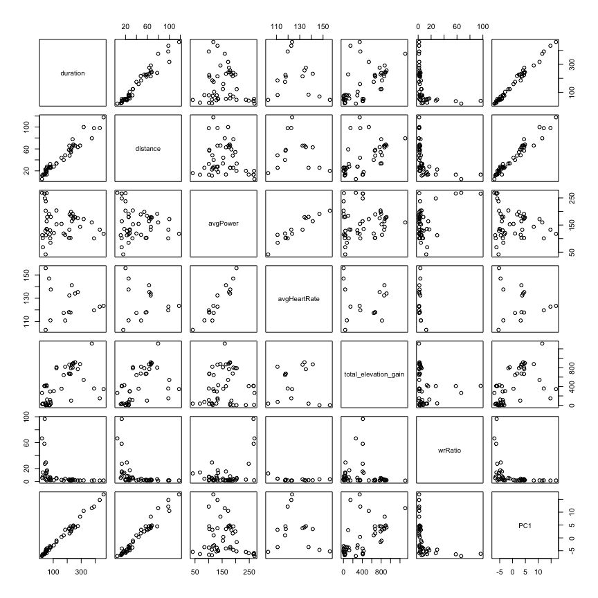
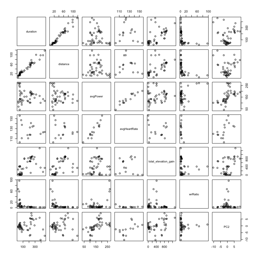
The principal components can then be used for further analyses or as features in further modelling
## Check which sessions have power data
has_power <- !is.na(athlete1_summaries$avgPower)
## Scatterplots of the first harmonic against session summaries (high correlation with distance and duration)
plot(cbind(data.frame(athlete1_summaries)[has_power, features], PC1 = athlete1_fpca$scores[, 1]))
## Scatterplots of the second harmonic against session summaries
plot(cbind(data.frame(athlete1_summaries)[has_power, features], PC2 = athlete1_fpca$scores[, 2]))
## etc
Please use the GoldenCheetahOpenData GitHub issue page to report any issues or suggest enhancements or improvements.
Please note that this project is released with a Contributor Code of Conduct. By participating in this project you agree to abide by its terms.
See the trackeR R package CRAN page for vignettes on the use of trackeR.
Frick, H., Kosmidis, I. (2017). trackeR: Infrastructure for Running and Cycling Data from GPS-Enabled Tracking Devices in R. Journal of Statistical Software, 82(7), 1–29. doi:10.18637/jss.v082.i07
Liversedge, M. (2020). GoldenCheetah OpenData Project. OSF. doi:10.17605/OSF.IO/6HFPZ


