ilantoren/UpdateOneField

Kotlin, Coroutines, and the Mongodb Coroutine Driver

Partitioning GDELT Data for further statistical analysis

This code:

This code has a simple plan:

• declare an aggregation (edit in Compass and export as Java)
• Use a coroutines to read the entire collection in batches and store that field change in a list
• Read the list and submit updates to the database in batches

Use-case: In The case of mongod and the data analyst I showed how Spark and the Mongodb Spark-Connector can be used to populate a database. The connection from MongoDB to other data tools programming environments makes it a very useful. Is MongoDB better than a RDBMS? I'll give that a qualified Yes because of Compass and the Aggregation framework. Having good tools for developing data queries is one of the things that sets MongoDB apart. And how does that relate to partitioning your data? When I had finished uploading all of my GDELT files to MongoDB I had a collection with 4M records. Not BigData, but certainly lots of data. Too much for running an analysis with R or Excel, but more importantly using a more manageable slice of data is faster and the initial questions about the data are not harmed by having a smaller dataset.

Is this a baseless claim?

For my initial analysis I was looking at AvgTone and the effects of Actor1CountryCode and GoldsteinScale.

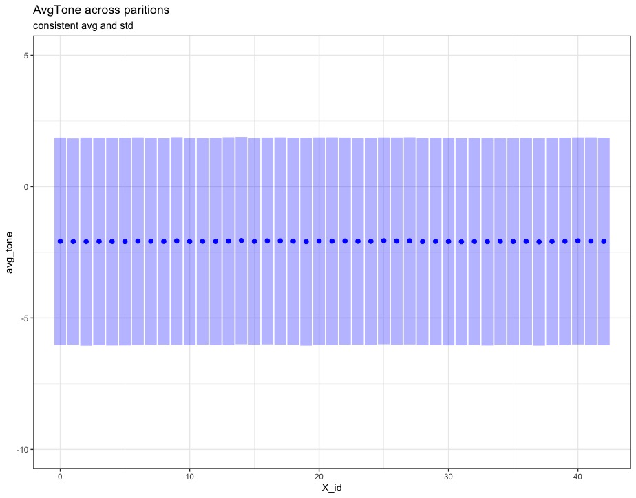
AvgTone: After partitioning and using an aggregation query I looked at the mean AvgTone and it's standard deviation
as follows:

from pymongo import MongoClient
import pandas as pd

client = MongoClient('mongodb://localhost:27017/')
result = client['gdelt']['data'].aggregate([{
  '$match': {
    'Actor1CountryCode': {
      '$exists': 0
    },
    'Actor1CountryCode': {
      '$exists': 1
    },
    'GoldsteinScale': {
      '$exists': 1
    },
    'AvgTone': {
      '$exists': 1
    }
  }
 }, {
   $group': {
     '_id': '$key',
     'count': {
     '$sum': 1
    },
     'avg_tone': {
     '$avg': '$AvgTone'
    },
     'sd_tone': {
     '$stdDevPop': '$AvgTone'
    },
     'avg_scale': {
     '$avg': '$GoldsteinScale'
    },
     'sd_scale': {
     '$stdDevPop': '$GoldsteinScale'
    }
  }
}], allowDiskUse=True)

df = pd.DataFrame(result)
df.to_parquet('gdelt_summary_stats')
df.to_csv( "gdelt_summary.csv")

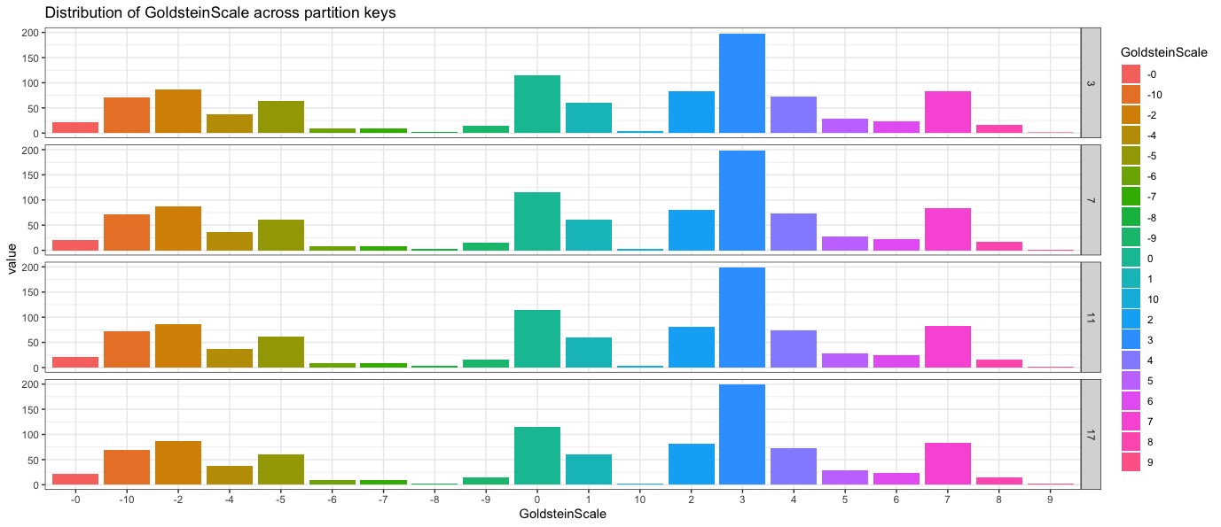
# CHECK BALANCE OF KEYS
keyq = '[
  {
    "$match": {
      "key": {
        "$in": [
          3, 7, 11, 17
        ]
      }, 
      "GoldsteinScale": {
        "$exists": 1
      }
    }
  }, {
    "$project": {
      "key": 1, 
      "GoldsteinScale": {
        "$toString": {
          "$round": [
            "$GoldsteinScale"
          ]
        }
      }
    }
  }
]'
client = mongo( collection="data", db="gdelt", url="mongodb://localhost")
key_data <- client$aggregate(keyq)
key_data %>% filter( is.na(GoldsteinScale) == FALSE) %>% group_by( key, GoldsteinScale ) %>% summarize( value=n(), .groups="rowwise") %>% group_by(key) %>% mutate(key, GoldsteinScale=as.factor(GoldsteinScale), value = round(1000*value/sum(value)) )  %>% as_tibble( colnames="key",rownames="GoldsteinScale", c( GoldsteinScale, value)) %>% ggplot(aes(x=GoldsteinScale, y=value, fill=GoldsteinScale)) + geom_col() ->p 
p + facet_grid(vars(key)) + labs( title="Distribution of GoldsteinScale across partition keys") + theme_bw()

What about the distribution of countries in different partitions?

#Examining distribution of CountryCodes in data by partition
library( mongolite)
library(dplyr)
library(arrow)
library(ggplot2)
library( tidyr)


aggregation = '
[
  {
    "$match": {
      "GoldsteinScale": {
        "$ne": null
      }, 
      "AvgTone": {
        "$ne": null
      }, 
      "Actor1CountryCode": {
        "$ne": null
      }, 
      "key": {
        "$in": [
          5, 9, 15, 19
        ]
      }
    }
  }, {
    "$project": {
      "Actor1CountryCode": 1, 
      "Actor2CountryCode": 1, 
      "Actor1Code": 1, 
      "GoldsteinScale": 1, 
      "AvgTone": 1, 
      "key": 1
    }
  }, {
    "$setWindowFields": {
      "partitionBy": "$Actor1CountryCode", 
      "output": {
        "count": {
          "$sum": 1
        }, 
        "tone_avg": {
          "$avg": "$AvgTone"
        }, 
        "scale_avg": {
          "$avg": "$GoldsteinScale"
        }, 
        "tone_std": {
          "$stdDevSamp": "$AvgTone"
        }
      }
    }
  }, {
    "$match": {
      "count": {
        "$gt": 1000
      }
    }
  }
]
'

client = mongo( collection="data", db="gdelt", url="mongodb://localhost")
country_data <- client$aggregate(aggregation)

country_data %>% ggplot( aes( x=Actor1CountryCode, fill=Actor1CountryCode)) +
     geom_bar(position = "identity") + ylim( 0, 5000) + facet_grid( vars(key)) +
     labs( title="Count of mentions of Actor1CountryCode by partition", caption="USA has been removed as count > 1000") + theme_bw()