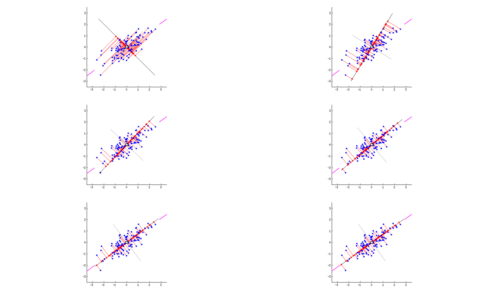
Principal Component Analysis is a process of computing the "Principal Components" and using them to perform changes in the data. It is a very popular algorithm that is often used in unsupervised learning for dimensionality reduction.
For example :- Suppose I have a dataset with 'm' data points that are of 'n' dimensions. Dimensionality reduction implies transforming those data points in such a way that they now have a reduced dimension of 'k' for all k less than n, without any significant loss of valuable information.
It can also be defined as projecting the data-points from an n-dimensional data space into a k-dimensional data space without losing the information they contain. This can be achieved through PCA.
Principal Components can be defined as vectors representing the directions along which the variances of the projected data are maximised. Principal components can be found out through methods like eigendecomposition.
Suppose we have a dataset X consisting of m examples and n features or we can say it as, we have m data points that are of n dimensions.
- Step 1 : Computing the Covariance Matrix of X
- For this we first need to compute the mean along each column that is the mean for every feature.
- Then we compute the deviations of my data points from the mean.
- Then we find out the covariance matrix using the mean and deviations we had calculated.
In our code we have used the Standard Scaler function to convert the data into a Standard Normal Distribution by reducing the mean to 0 and the standard deviation to 1.
This helps us reduce the computation time and increses the computation efficiency.
- Step 2 : Finding the Eigen vectors and the Eigen values of the Covariance matrix or undergoing Eigendecomposition.
- We find the Eigen vectors of the covariance matrix of X to diagonalise the covariance matrix of the dataset transformed from X. The Eigen vectors give me the direction along which the transformation of my dataset X took place. The Eigen values contained in the diagonal elements give me the magnitude of the transformation.
- We find the Eigen vectors of the covariance matrix of X to diagonalise the covariance matrix of the dataset transformed from X. The Eigen vectors give me the direction along which the transformation of my dataset X took place. The Eigen values contained in the diagonal elements give me the magnitude of the transformation.
- Step 3 : Calculating the cumulative explained variance.
- The cumulative explained variance calculated explains how much variance does each feature retain.
- Step 4 : Deciding on how many principal components to consider
- We can do this by setting a threshold like the components who retain more than 95-99% of the total variance can be considered as the principal components.
- We can do this by setting a threshold like the components who retain more than 95-99% of the total variance can be considered as the principal components.
Once we are done deciding on the number of Principal Components to use, we can then reduce the dimension of our original dataset from n to the number of principal components selected.
We then project our data points onto the principal components and finally we get a matrix where the columns specify the values of the projected data.
