This repository contains sample code to train and visualise a simple Convolutional Neural Network to classify the Fashion MNIST dataset using TensorFlow 2.x. Whilst the network architecture is a simple Sequential model (details below), the goal is to highlight the ability to visualise the model as it classifies input images.
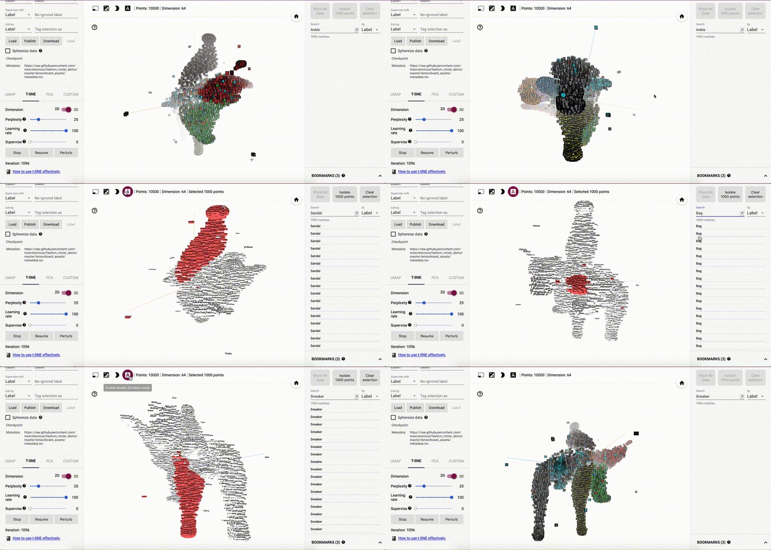 👉 Live demo of embedding vectors on Tensorboard.
- Summary
- Usage
- Model Structure
- Network Layer Visualisations
- Embedding Vectors
- Live Demo
- Further Reading
- Experimental
- Licence
- A Convolutional Neural Network is trained (see train.py) to classify images from the Fashion MNIST dataset. The main features showcased here:
- ModelCheckpoint callback saves only when validation loss (
val_loss) improves - EarlyStopping callback stops training when validation loss (
val_loss) stops improving - Dropout to limit overfitting
- GlobalAveragePooling to simplify feature extraction along with spatial invariance
- Tensorboard logging of Images, Histograms and Distributions along with Scalars like
accuracy&loss
- ModelCheckpoint callback saves only when validation loss (
- Classification of a new image (passed in using a command line argument or one of the sample images located in sample_images) using a trained model (:point_up:) using classify.py.
- Exporting test images from dataset for visualisation in Tensorboard Projector
Details about the dataset can be found here. Briefly, each image is 28 x 28 pixels and is one of ten different types of fashion categories (Shirt, Dress, Sneakers etc). The classification task is to train a model that can take one of these images as input and classify it into one of the existing categories. After training several visualisations are generated to see the model's learning.
These visualisations cover:
- Transformations to input image: transforming the input image before it is passed as input to the network
- Class activation map: a heatmap overlaid on the input image to see where the network is paying 'Attention'
- Confusion matrix: a matrix showing the model's performance on the different classes compared to the true classes
- Layer activations: output of each feature map of each layer in the network for a single input
- Live Demo: exporting embedded vectors for each input in the test set for visualistion and analysis in Tensorboard Projector
A Python virtual environment (see this guide for more information) is recommended when installing Python libraries. This prevents system-wide installs and allows each environment to function as a sandbox.
A full list of requirements can be found in requirements.txt. Additionally graphviz is required for plotting the model's structure (this is an OS level install). The main dependencies of note are:
- Python 3.7
- TensorFlow 2.x
- pillow (used for image loading, greyscale conversions and resizing)
- pydot & graphviz (used for plotting model structure)
All dependecies can be installed by running the following on the command line:
## execute from project root folder
pip install -r requirements.txt
Note: graphviz needs to be installed on the system
Simply run (from the project root path):
PYTHONPATH=fashion_mnist_vis python fashion_mnist_vis/train.pyThe trained model will be saved in the project root with the filename model.h5.
To classify one of the sample images:
PYTHONPATH=fashion_mnist_vis python fashion_mnist_vis/classify.py sample_images/black_bag.jpg --saved_model model.h5 --save_plotsHere the saved model (model.h5) and image (black_bag.jpg) can be substituted as needed. All visualisations will be stored in the visualisations folder. To avoid plotting each time and only classify the image, remove the --save_plots argument from the command. As the model expects a 28 x 28 image, the input image will be resized to 28 x 28.
Note: Input images in the training set are square with the object centered. For best results, new images should be similar.
Embedding vectors (see below for more details) are exported for visualising in Tensorboard Projector.
First export assets using:
PYTHONPATH=fashion_mnist_vis python fashion_mnist_vis/tensorboard_visualise.py --saved_model model.h5This will store necessary files in the tensorboard_assets folder.
Second, start a CORS server using the provided tensorboard_assets/serve_assets.py script:
cd tensorboard_assets
python serve_assets.py
This will start a simple webserver to serve the exported embedding vector data (with CORS enabled) on port 8000.
Finally, go to http://projector.tensorflow.org/?config=http://localhost:8000/config.json in a browser to view the embedded vectors in Tensorboard Projector.
| Summary | Graph Diagram |
|---|---|
| A simple, sequential Convolutional Neural Network with Batch Normalisation, a Global Average Pooling layer (for Attention) and Dropout. Note there are no fully connected layers in this network. This model achieved an accuracy of 92.07% on the test set. It is expected that a model with skip connections as popularised by the ResNet-50 architecture would improve the classification capabilities. However the visualisation of such a network with merge layers would be more difficult and harder to grok for people starting out. |  |
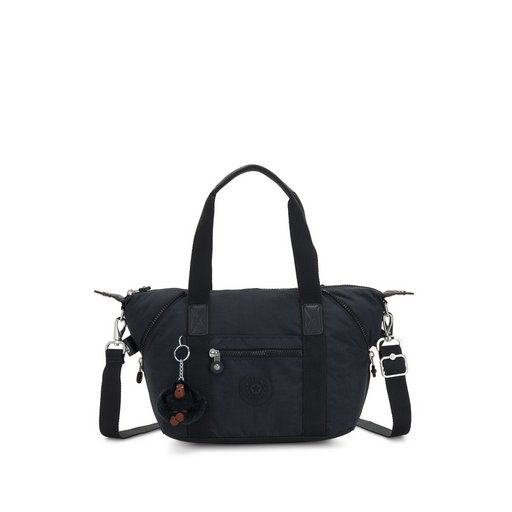
A black handbag from Argos is chosen as our input - KIPLING Black Art Mini Handbag - One Size
Model classification: Bag with a score of 0.9213.
Image is from an Argos product page so out of the train and test datasets. This is a crucial validation of the model's ability to generalise and work on data that's not restricted to the dataset itself. CNNs have tremendous memorisation capabilities and seeing its ability to correctly classify data that is from a different source (but still in line with the training dataset's patterns) is fundamental to proving its effectiveness.
The model only accepts greyscale images with a resolution of 28 x 28 so all input images will need to be
- converted to greyscale
- resized to
28 x 28
before they can be sent to the model.
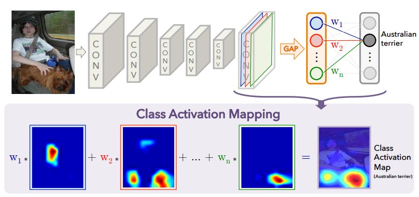
A class activation map for a particular category indicates the discriminative image regions used by the CNN to identify that category. The procedure for generating a CAM (from Learning Deep Features for Discriminative Localization) is illustrated below:
Source: http://cnnlocalization.csail.mit.edu/
| Input To Model | Class Activation Map |
|---|---|
 |
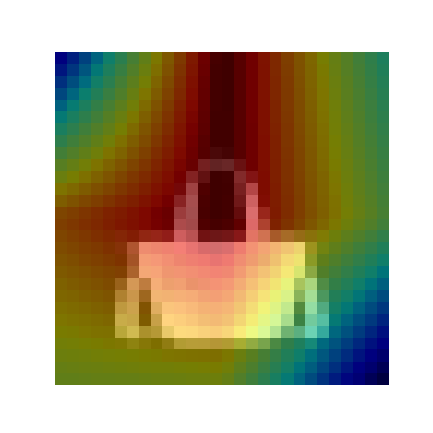 |
Looking at the activation map 🤔, it appears the model is paying attention to the handle of the bag in making it's classification (along with the absence of anything above the handle).
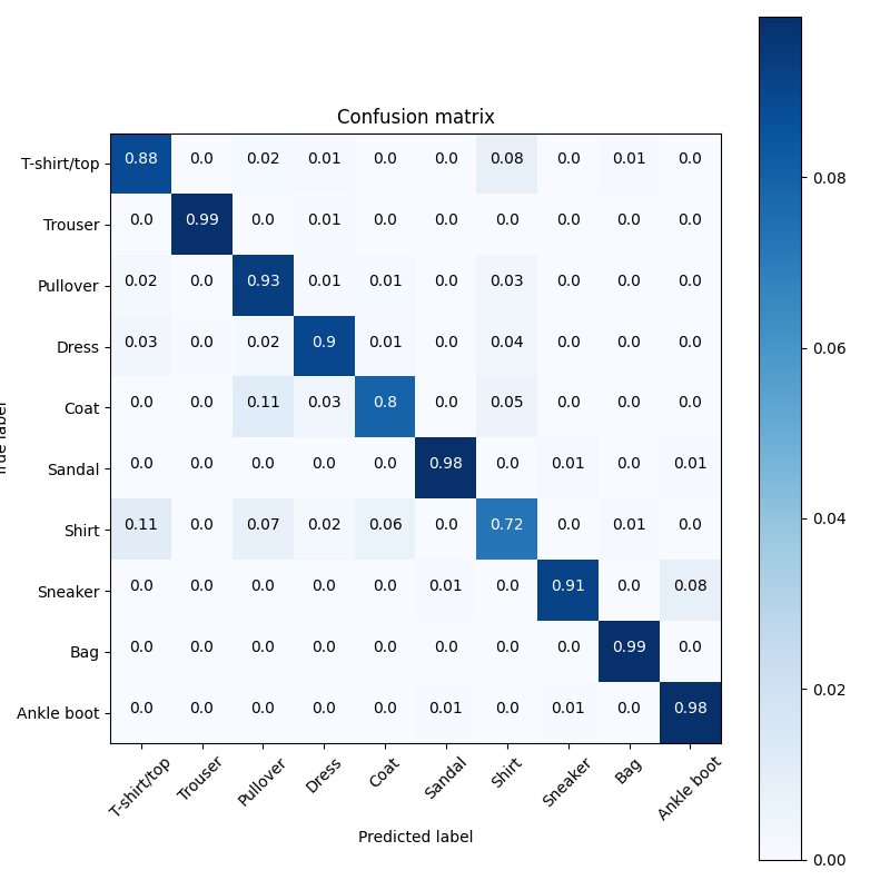
(From Wikipedia) a confusion matrix is a specific table layout that allows visualization of the performance of a classification algorithm. It allows for a comparison of the model's ability to correctly, or incorrectly, classify certain classes. Rows represent the true class labels whilst the columns represent the model's predictions.
This matrix provides visibility on the classes the model is 'struggling' to classify correctly. In this case the 'Shirt' & 'Coat' classes have the worst accuracy (72% & 80% respectively). A large number (11%) of 'Shirt' images are misclassified as 'T-shirt/top'. Whilst understandable as the distinction between these classes is not as stark as the other classes, the model is still expected to perform reasonably on these classes. Conversely, the 'Trousers' & 'Bag' classes have the best accuracy (99%). Data augmentation is likely to help improve the model's performance, especially on the former pair of classes.
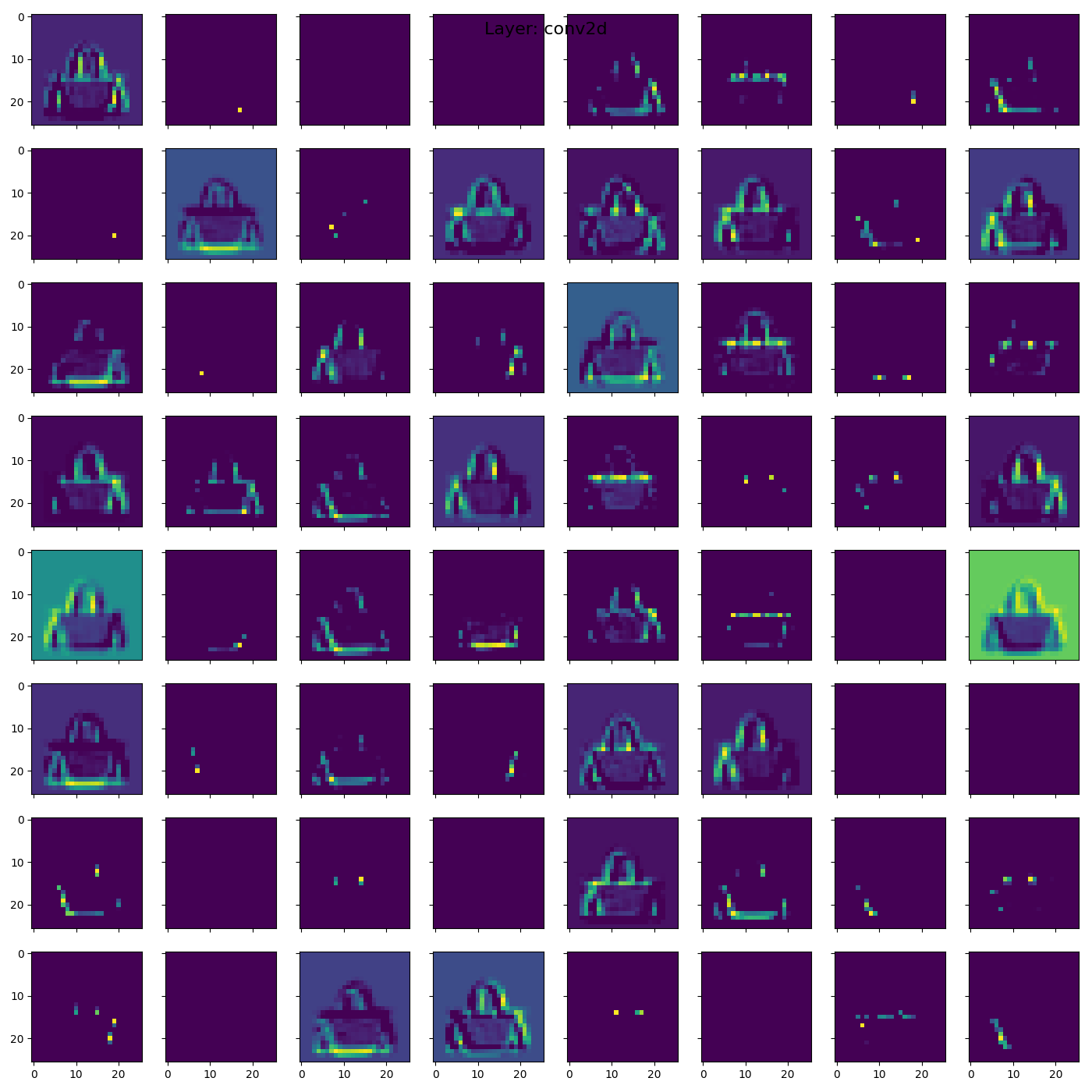
The transformed image (as detailed above) passes through the network and each of the feature maps in each layers extracts some features from it. The lower layers of the network (CNN Layer 1 & 2 below 👇) typically end up as edge detectors. Specifically they look for certain kinds of edges that are of 'use' to the layers deeper in the network. Layers futher down in the network use these features to activate when certain criteria is met. For example, the first few layers of feature maps might activate on a pair of curved edges near the top middle of the image (like seen in the handle of a bag. Higher layers will then activate when seeing these features to indicate that there is strong probability that a bag's handle is visible in the image. Eventually the final few layers will activate to indicate a 'Bag' class if all the collection of features most closely match a bag (a handle, a solid shape in the middle etc).
| CNN Layer 1 | CNN Layer 2 |
|---|---|
 |
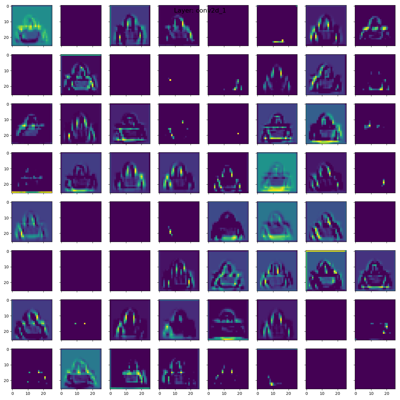 |
☝️ We see 64 feature maps in the two layers above showing different activations for the bag. Invariably, some of these will be blank as they only activate when detecting edges of other classes (like 'Ankle Boot' or 'Sneaker').
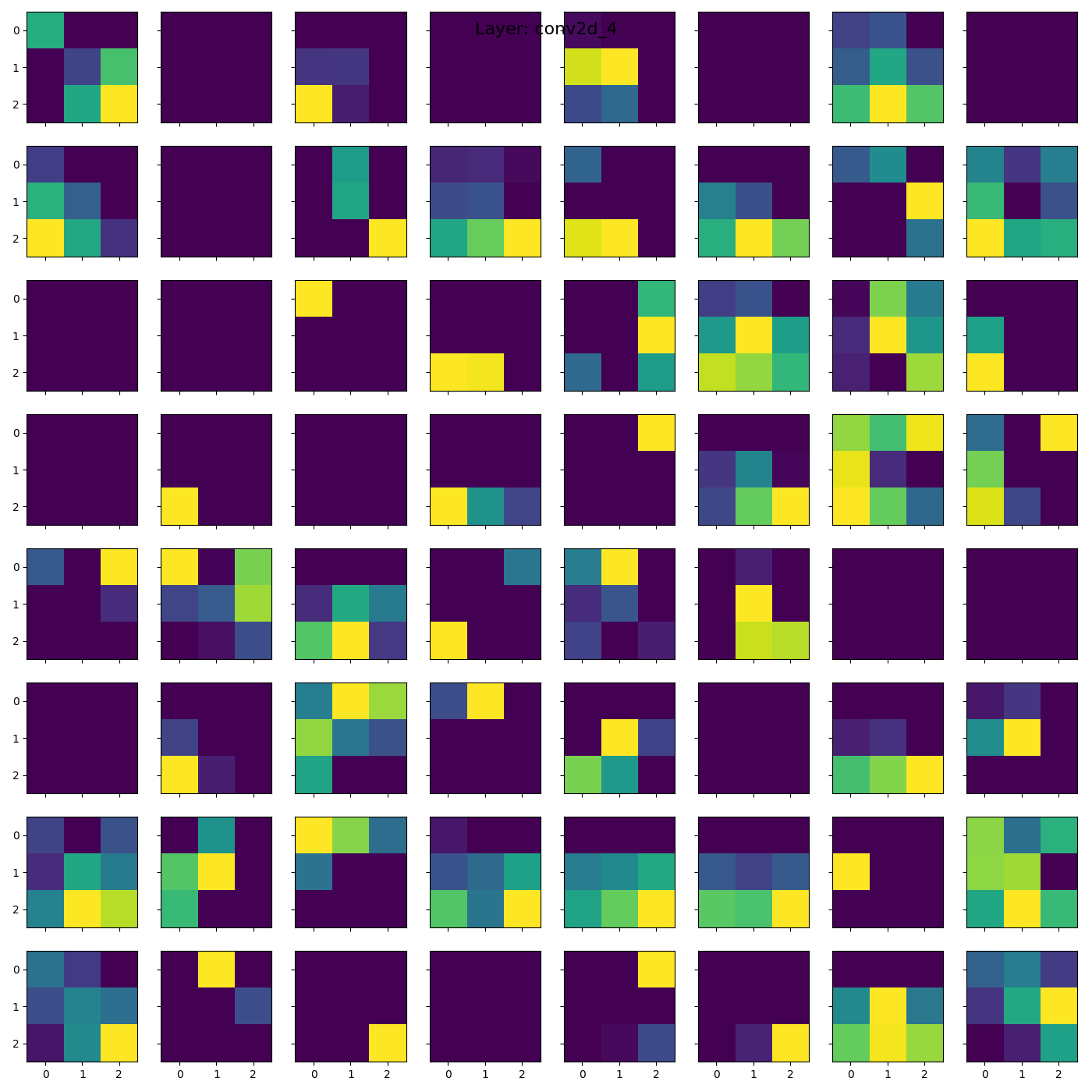
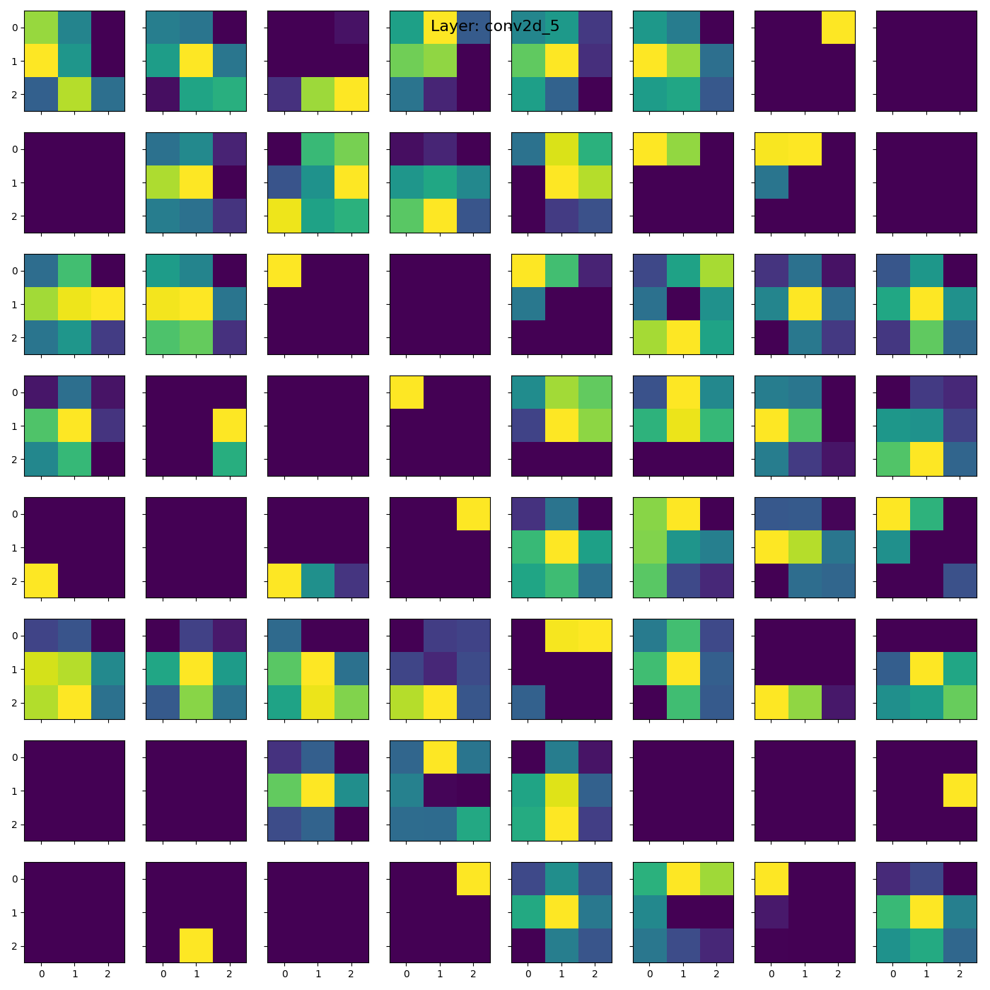
👇 The last few convolutional layers (5 & 6) do not bear any recognisable resemblance to the input image, however they are showing activations on groups of features.
| CNN Layer 5 | CNN Layer 6 |
|---|---|
 |
 |
The activations from the previous layer are averaged using a Global Average Pooling layer. Activations from this layer provide the embedding vector (see next section) that the model uses to make the final classification.
| Global Average Pooling | Dense (Final) |
|---|---|
 |
 |
Note: the Dropout layer is not visualised as it is only used whilst training the network. When making a prediction the network does not perform any function.
An embedding vector provides a vectorised representation of an input datapoint. In the case of this model each input datapoint can be thought of a 28 x 28 = 784 dimensional vector. As this image passes through the network's layers, it is transformed until it is ultimately a 64 dimension vector. This is the penultimate layer in the network and contains enough information about the datapoint to allow the final layer to perform the classification. Examining the quality of these vectors can provide insight into the strengths and weaknesses of the model. For instance,
- does the model classify some images more easily than others?
- is there a pattern or common feature amongst images the model is struggling to classify correctly?
- is the embedding vector carrying any meaningful representation?
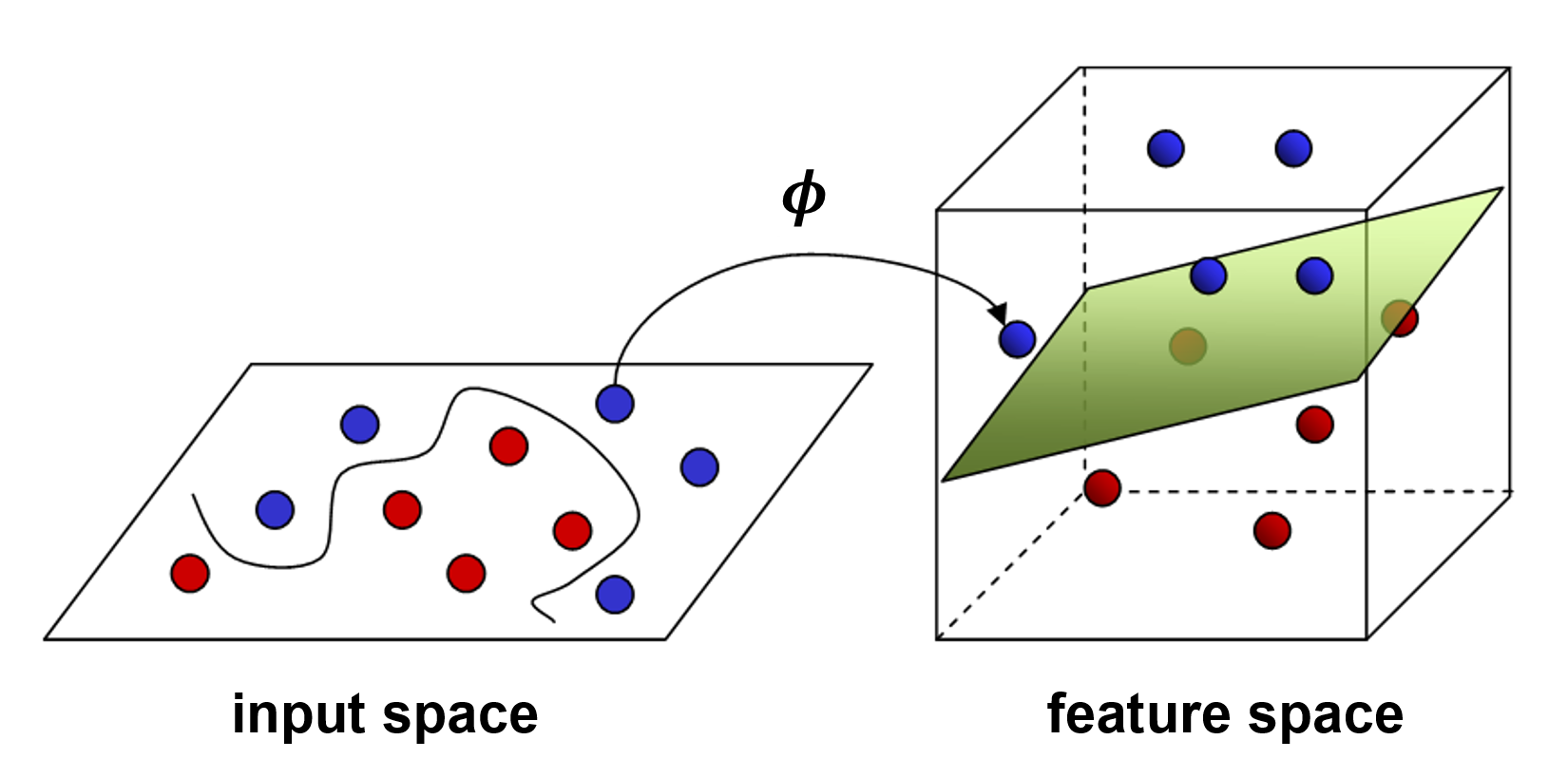
When making classifications, the model makes decisions about the class of the image based on the embedding vector. A clear separation between two classes in the embedding vector space makes the task simpler for the model. The separation boundary is also known as a decision boundary or a hyperplane.
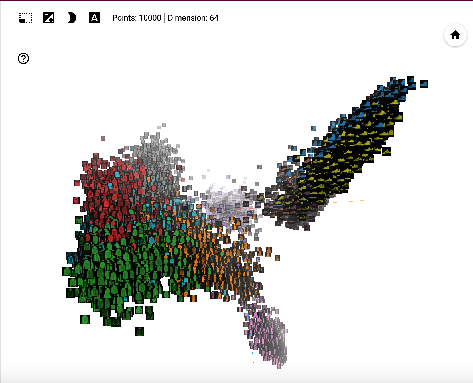
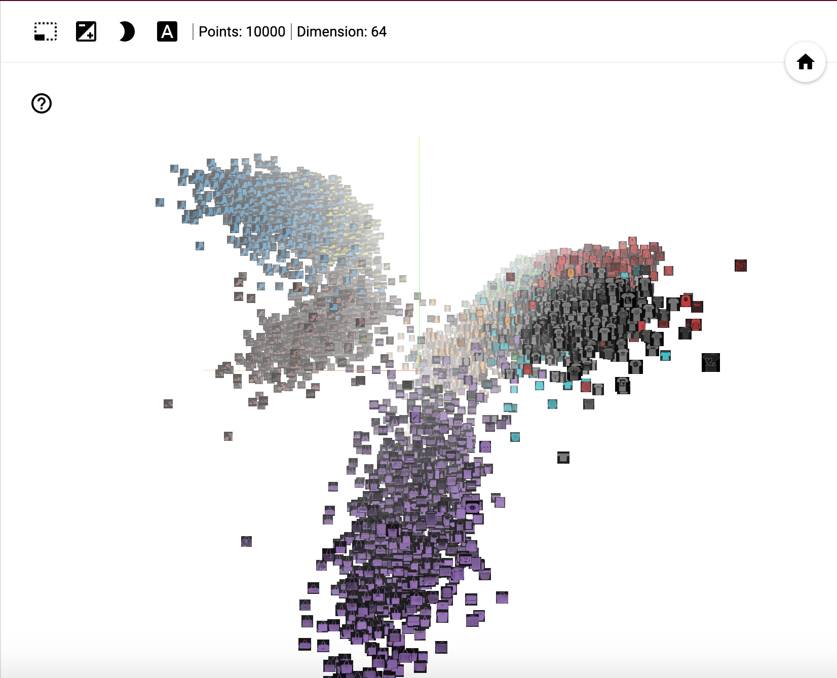
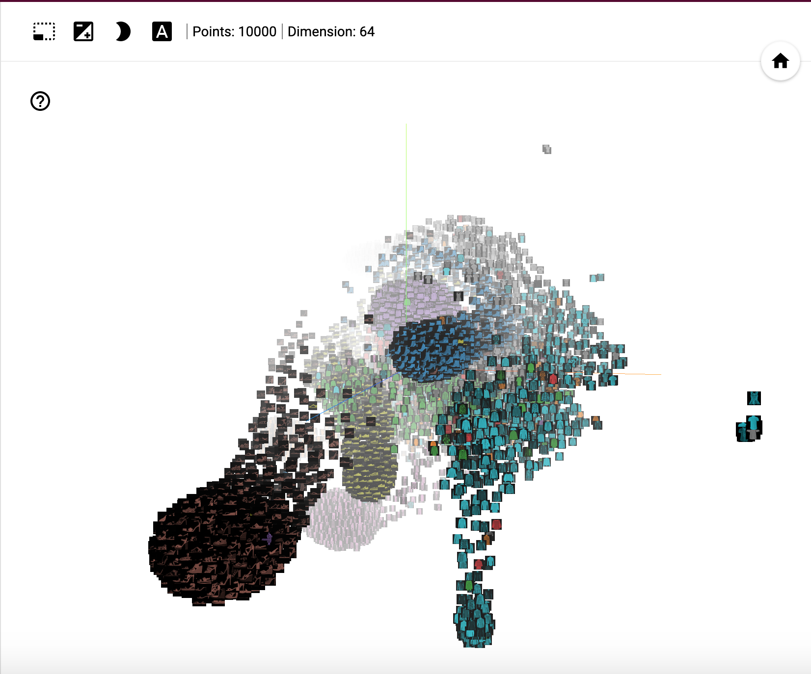
The following visualisations are aimed at examining these embedding vectors to understand how the model is 'representing' the images. As we cannot visualise a 64 dimension vector directly, we have to perform dimensionality reduction to bring the dimensionality down to two or three dimensions. Each dimensionality reduction algorithm has its tradeoffs. PCA and t-SNE will be used.
Each datapoint represents a single image. It's important to focus on the relative positioning of the data instead of the absolute values. For instance, the three dimensions don't carry any special meaning, they simply represent the most appropriate dimensions to visualise the data (the definition of what constitutes 'most appropriate' is specific to each individual algorithm). When examining the visualisations, it is useful to see the separation of the different classes.
Classes that have a clear hyperplane or decision boundary separating them are easier for the model to classify (the creation of the hyperplane is the direct result of the training process). These hyperplanes can be viewed as distinct decision boundaries. However, where a clear hyperplane is not visible (like between 'Coat' and 'Shirt') the model will struggle to accurately distinguish between the different classes.
Source: Dealing with nonlinear decision boundaries
In order to get a sense of the higher dimensional positioning of the datapoints (in this case 64D), a few algorithms are used to provide a mapping between the higher (64D) and lower (3D) dimensions whilst retaining certain characteristics about the datapoints.
PCA is a simple, powerful algorithm to reduce a high dimensional vector to low dimenions. In the images below, the 64 dimension embedding vector is reduced to 3 dimensions and plotted by Tensorboard. A quick and easy starting point for analysing high dimensional data it does struggle to deal with non-linearity in the higher dimensions.
| Image 1 | Image 2 |
|---|---|
 |
 |
t-SNE is a non-deterministic algorithm to visualise high dimenional data in lower dimensions whilst retaining spatial information. See this excellent article on how to effectively use t-SNE. It's important to note that unlike PCA, t-SNE is not a generalised function that takes high dimensional data and output low dimensional equivalents. Instead, it provides a mapping for known datapoints only.
| Image 1 | Image 2 |
|---|---|
 |
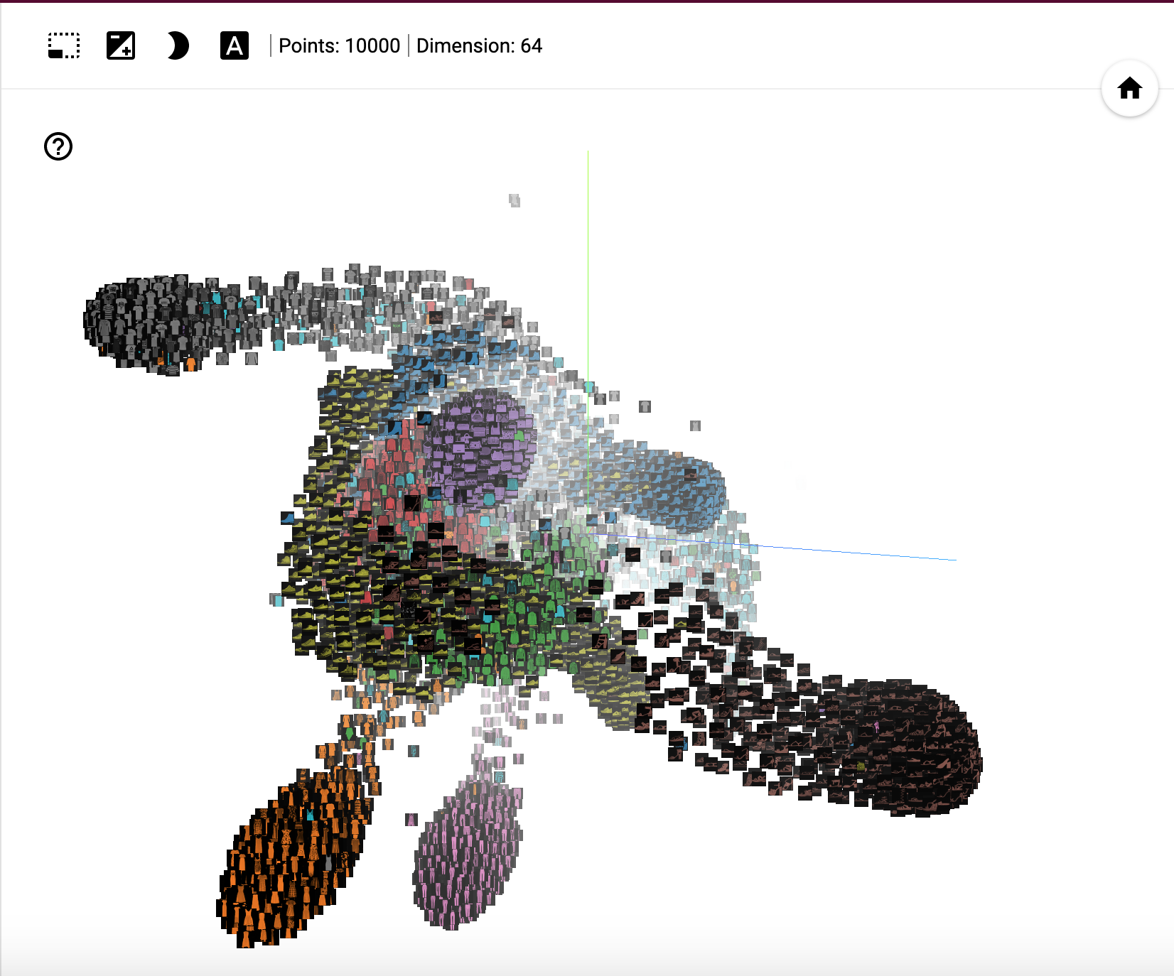 |
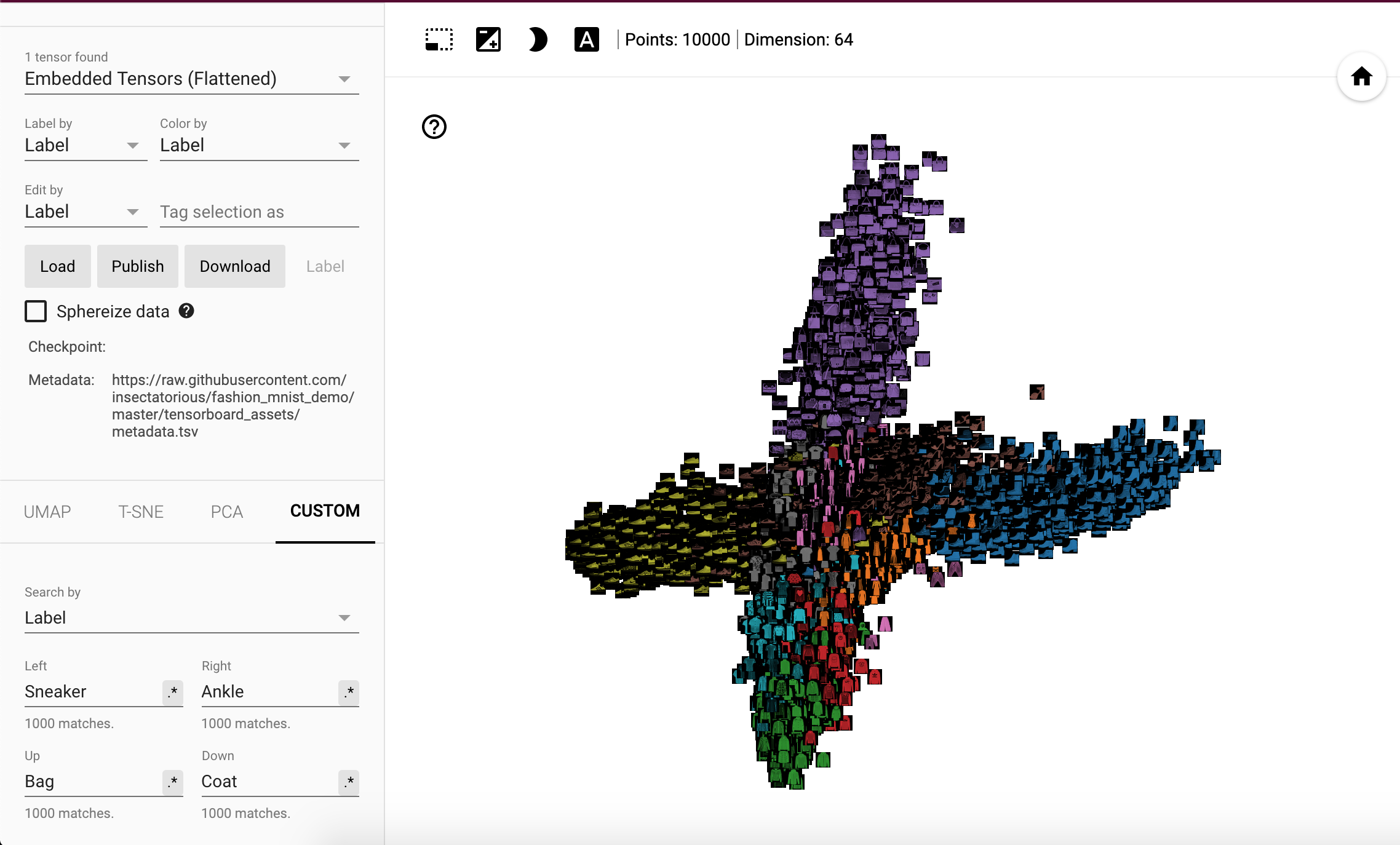
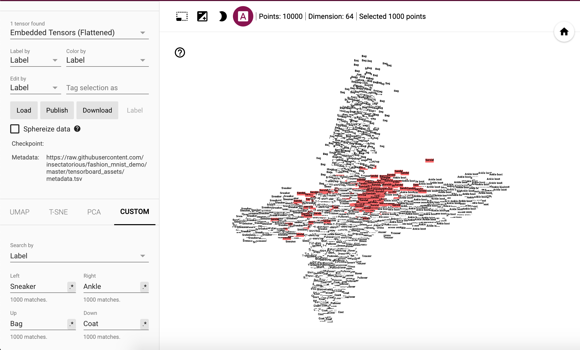
Tensorboard allows users to map projections for datapoints matching certain criteria against each other. In the following examples datapoints matching the 'Sneaker' vectors are projected to the left and those matching 'Ankle' are projected to the right. This can be interpreted as, the more to the left or right a data point is, the more similar it is to a 'Sneaker' or 'Ankle' datapoint. Similarly, 'Bag' and 'Coat' are projected up and down respectively.
The image below 👇 shows an example of 'Sandal' images highlighted. Most of them are closer to the right making them similar to 'Ankle Boot' but a number of them are also seen on the left making these similar to 'Sneakers'.
View the embedded vectors on Tensorboard. Works best in Chrome or Firefox.
The vectors visualised here are exported using the model model.h5, saved in this repository.
- Applied Deep Learning - Part 4: Convolutional Neural Networks - Towards Data Science
- Conv Nets: A Modular Perspective - Chris Olah's Blog
- Understanding Convolutions - Chris Olah's Blog
- Neural Networks, Manifolds, and Topology - Chris Olah's Blog
- Transfer Learning With A Pretrained ConvNet - Tensorflow Official Guide
Code with interesting results is located in the ./fashion_mnist_vis/experimental folder.
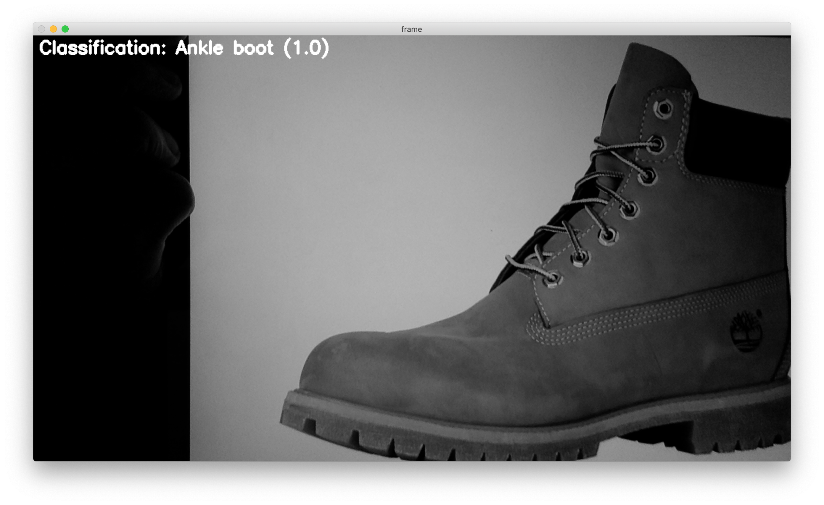
For instance using the webcam to classify a livestream using the trained Fashion MNIST model. See the Experimental README for more information.
GNU General Public License v3.0
Permissions of this strong copyleft license are conditioned on making available complete source code of licensed works and modifications, which include larger works using a licensed work, under the same license. Copyright and license notices must be preserved. Contributors provide an express grant of patent rights.


