Note: This fork contains proposed updates to the Quantum Economic Development Consortium's benchmark suite. To use this repository to calculate #AQ, please see the instructions here.
This repository contains a collection of prototypical application- or algorithm-centric benchmark programs designed for the purpose of characterizing the end-user perception of the performance of current-generation Quantum Computers.
The repository is maintained by members of the Quantum Economic Development Consortium (QED-C) Technical Advisory Committee on Standards and Performance Metrics (Standards TAC).
Important Note -- The examples maintained in this repository are not intended to be viewed as "performance standards". Rather, they are offered as simple "prototypes", designed to make it as easy as possible for users to execute simple "reference applications" across multiple quantum computing APIs and platforms. The application / algorithmic examples are structured using a uniform pattern for defining circuits, executing across different platforms, collecting results, and measuring the performance and fidelity in useful ways.
A wide variety of "reference applications" are provided. At the current stage in the evolution of quantum computing hardware, some applications will perform better on one hardware target, while a completely different set may execute better on another target. They are designed to provide for users a quantum "jump start", so to speak, eliminating the need to develop for themselves uniform code patterns that facilitate quick development, deployment and experimentation.
The QED-C committee which developed these benchmarks released a pre-print of a paper describing the theory and methdology supporting this work at Application-Oriented Performance Benchmarks for Quantum Computing.
See the Implementation Status section below for the latest report on benchmarks implemented to date.
The repository is organized at the highest level by specific reference application names. There is a directory for each application or algorithmic example, e.g. quantum-fourier-transform, which contains the the bulk of code for that application.
Within each application directory, there is a second level directory, one for each of the target programming environments that are supported. The repository is organized in this way to emphasize the application first and the target environment second, to encourage full support across platforms.
The directory names and the currently supported environments are:
    qiskit      -- IBM Qiskit
    cirq        -- Google Cirq
    braket      -- Amazon Braket
The goal has been to make the implementation of each algorithm identical across the different target environments, with processing and reporting of results as similar as possible. Each application directory includes a README file with information specific to that application or algorithm. Below we list the benchmarks we have implemented with a suggested order of approach; the benchmarks in levels 1 and 2 are more simple and a good place to start for beginners, while levels 3 and 4 are more complicated and might build off of intuition and reasoning developed in earlier algorithms.
Complexity of Benchmark Algorithms (Increasing Difficulty)

    1: Deutsch-Jozsa, Bernstein-Vazirani, Hidden Shift
    2: Quantum Fourier Transform, Grover's Search
    3: Phase Estimation, Amplitude Estimation
    4: Monte Carlo, Hamiltonian Simulation, Variational Quantum Eigensolver, Shor's Order Finding
In addition to the application directories at the highest level, there several other directories or files with specific purpose:
    _common                      -- collection of shared routines, used by all the application examples
    _doc                         -- detailed DESIGN_NOTES, and other reference materials
    _containerbuildfiles         -- build files and instructions for creating Docker images (optional)
    _setup                       -- information on setting up all environments

    benchmarks-*.ipynb.template  -- Jupyter Notebook templates
The prototype benchmark applications are easy to run and contain few dependencies. The primary dependency is on the Python packages needed for the target environment in which you would like to execute the examples.
In the _setup folder you will find a subdirectory for each of the target environments that contains a README with everything you need to know to install and configure the specific environment in which you would like to run.
Important Note:
The suite of application benchmarks is configured by default to run on the simulators
that are typically included with the quantum programming environments.
Certain program parameters, such as maximum numbers of qubits, number of circuits
to execute for each qubit width and the number of shots, are defaulted to values that
can run on the simulators easily.

However, when running on hardware, it is important to reduce these values to account
for the capabilities of the machine on which you are executing. This is especially
important for systems on which one could incur high billing costs if running large circuits.
See the above link to the _setup folder for more information about each programming environment.
The benchmark programs may be run manually in a command shell. In a command window or shell, change directory to the application you would like to execute. Then, simply execute a line similar to the following, to begin execution of the main program for the application:
    cd bernstein-vazirani/qiskit
    python bv_benchmark.py
This will run the program, construct and execute multiple circuits, analyze results and produce a set of bar charts to report on the results. The program executes random circuits constructed for a specific number of qubits, in a loop that ranges from min_qubits to max_qubits (with default values that can be passed as parameters). The number of random circuits generated for each qubit size can be controlled by the max_circuits parameter.
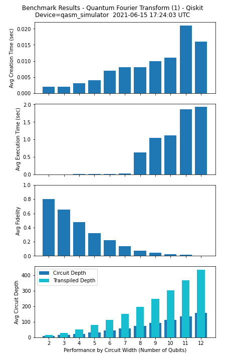
As each benchmark program is executed, you should see output that looks like the following, showing the average circuit creation and execution time along with a measure of the quality of the result, for each circuit width executed by the benchmark program:
Alternatively you may use the Jupyter Notebook templates that are provided in this repository.
Simply copy and remove the .template extension from the copied ipynb template file.
There is one template file provided for each of the API environments supported.
In the top level of this repo, start your jupyter-notebook process. When the browser listing appears, select the desired notebook .ipynb file to launch the notebook.
There you will have access to a cell for each of the benchmarks in the repository, and may "Run" any one of them independently and see the results presented there.
There is support provided within the Jupyter Notebook for the Qiskit versions of the benchmarks to enable certain compiler optimizations. In the first cell of the notebook there is a variable called exec_options where several of the built-in Qiskit compiler optimizations may be specified.
The second cell of the Jupyter notebook contains commented code with references to custom coded Qiskit compiler optimizations as well as some third-party optimization tools. Simply uncomment the desired optimizations and rerun the notebook to enable the optimization method. The custom code for these optimizations is located in the _common/transformers directory. Users may define their own custom optimizations within this directory and reference them from the notebook.
Applications are often deployed into Container Management Frameworks such as Docker, Kubernetes, and the like.
The Prototype Benchmarks repository includes support for the creation of a unique 'container image' for each of the supported API environments. You can find the instructions and all the necessary build files in a folder at the top level named _containerbuildfiles.
The benchmark program image can be deployed into a container management framework and executed as any other application in that framework.
Once built, deployed and launched, the container process invokes a Jupyter Notebook from which you can run all the available benchmarks.
- Creation Time: time spent on classical machine creating the circuit and transpiling.
- Execution Time: time spent on quantum simulator or hardware backend running the circuit. This only includes the time when the algorirhm is being run and does not inlcude any of the time waiting in a queue on qiskit and cirq. Braket does not currently repor execution time, and therefore does include the queue time as well.
- Fidelity: a measure of how well the simulator or hardware runs a particular benchmark, on a scale from 0 to 1, with 0 being a completely useless result and 1 being perfect execution of the algorithm. The math of how we calculate the fidelity is outlined in the file
_doc/POLARIZATION_FIDELITY.md. - Circuit/Transpiled Depth: number of layers of gates to apply a particular algorithm. The Circuit depth is the depth if all of the gates used for the algorithm were native, while the transpile depth is the amount of gates if only certain gates are allowed. We default to
['rx', 'ry', 'rz', 'cx']. Note: this set of gates is just used to provide a normalized transpiled depth across all hardware and simulator platforms, and we seperately transpile to the native gate set of the hardware. The depth can be used to help provide reasoning for why one algorithm is harder to run than another for the same circuit width. This metric is currently only available on the Qiskit implementation of the algorithms.
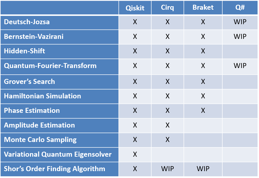
Below is a table showing the degree to which the benchmarks have been implemented in each of the target platforms (as of the last update to this branch):

