Machine Learning with Python

Implementation of Sklearn and Deep Learning models.

Everything about Regression

Started to mathematically improve the navigation methods based on astronomy during age of exploration in 1700s.

Simply described: Regression is a statistical method used to understand the relationship between a dependent variable and one or more independent variables. The goal is to predict the value of the dependent variable based on the values of the independent variables.

Roger Cotes (1722): He discovers that by combining observations yields better estimate of true value.
Tobias Mayer (1750): He explored averaging different results for studying moon.
Adrien-Marie Legendre (1805): Least Squares Method - First public exposition on linear regression. (He also introduced the basic properties of elliptic integrals, beta functions and gamma functions.)
Carl Friedrich Gauss (1809): He claimed that he have invented least-squares back in 1795! during orbits calculation of celestial bodies. He is referred as the foremost of mathematicians.

OLS

OLS stands for Ordinary Least Squares. It is a method for estimating the parameters of a linear regression model.

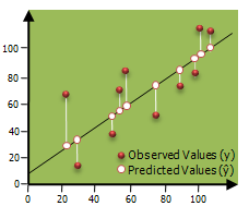
The goal of OLS is to find the values of the parameters (such as the slope and intercept) that minimize the sum of the squared differences between the predicted values (based on the model) and the actual observed values.

This method is called "least squares" because it finds the set of parameters that minimize the sum of the squared errors.It finds the line of best fit that minimizes the sum of the squared residuals (the distances between the line and the actual data points) and also it is widely used for Linear Regression.

We know that, y = mx + c is simple straight line equation with m as the slope and b as y-axis intercept. Here only one feature is possible: which is x.
In generalised form: If we have x1, x2, x3, ..... xn as the feature, then each feature should have some beta coefficient associated with it. Hence, the equation can be written as:

$\hat{y}$ = β₀ x₀ + β₁ x₁ +β₂ x₂ + ... + β_n x_n
We have hat over $\hat{y}$ because it is estimation and not actual value. There is usually no set of betas to create a perfect fit to y!

Pearson Correlation Coefficient

The Pearson correlation coefficient, also known as Pearson's r, is a measure of the linear association between two variables. The coefficient takes a value between -1 and 1, with -1 indicating a perfect negative correlation, 1 indicating a perfect positive correlation, and 0 indicating no correlation. A positive correlation means that as one variable increases, the other variable also tends to increase, and similarly, as one variable decreases, the other variable also tends to decrease. A negative correlation means that as one variable increases, the other variable decreases, and vice versa.

The coefficient can be calculated by dividing the covariance of the two variables by the product of their standard deviations. The result of this calculation is a standardized measure that allows for comparisons of correlation across different data sets.

It's important to note that correlation does not imply causation, meaning that just because two variables are correlated it does not mean that one variable is causing the other variable.

r = cov(X, Y) / (std(X) * std(Y))

where X and Y are the two variables, cov(X, Y) is the covariance of X and Y, and std(X) and std(Y) are the standard deviations of X and Y, respectively.

The Pearson correlation coefficient and linear regression are related because they both measure the linear association between two variables. The correlation coefficient (r) measures the strength and direction of the linear relationship between two variables, while linear regression estimates the equation of the line that best describes the relationship between the two variables.

In a simple linear regression model, the goal is to find the line that best fits the data, where the line is represented by the equation:

y = b0 + b1*x

Where y is the dependent variable, x is the independent variable, b0 is the y-intercept and b1 is the slope of the line.

The slope of the line (b1) in a simple linear regression model is equal to the Pearson correlation coefficient (r) multiplied by the ratio of the standard deviation of the dependent variable to the standard deviation of the independent variable.

b1 = r * (std(Y) / std(X))

Limitation of Linear Regression

Anscombe's Quartet: Each graph resulted in same regression line.

Linearity Assumption: Regression analysis assumes that the relationship between the independent and dependent variables is linear. If the relationship is non-linear, the results of the regression analysis may not be accurate.
Outliers: Regression analysis is sensitive to outliers, which are extreme values that are far from the other data points. Outliers can have a large impact on the results of the regression analysis and can lead to inaccurate conclusions.
Multicollinearity: Regression analysis assumes that the independent variables are not highly correlated with each other. When two or more independent variables are highly correlated, it can be difficult to determine the unique effect of each variable on the dependent variable.
Non-constant variance: Regression analysis assumes that the variance of the errors is constant across the range of the independent variable. If the variance is not constant, the results may be biased.
Non-normality of errors: Regression analysis assumes that the errors follow a normal distribution. If the errors do not follow a normal distribution, the results of the regression analysis may not be accurate.

But, How we can scale our simple regression for `n` numbers of features:

We can use gradient descent to solve a cost function to calculate Beta Values. The best-fit line minimizes the squared error.

Average squared error: (1/m) ( y^j - y^{^}^j) ²

Here y^{^}^j is predicted value of y for feature j while y^j is actual value of y for j. Assuming total m observations.

ishwar6/machine_learning