Sign Language Detection

How to Run

Setup Environment

$ git clone https://github.com/its-Kumar/signlang_project.git
$ cd signlang_project
$ pip install virtualenv
$ virtualenv venv
$ source venv/bin/activate

Install requirements

$ pip install -r requirements.txt

Running the application

$ python src/main.py

Image Classification of an American Sign Language Dataset

The American Sign Language alphabet contains 26 letters. Two of those letters (j and z) require movement, so they are not included in the training dataset.

kaggle

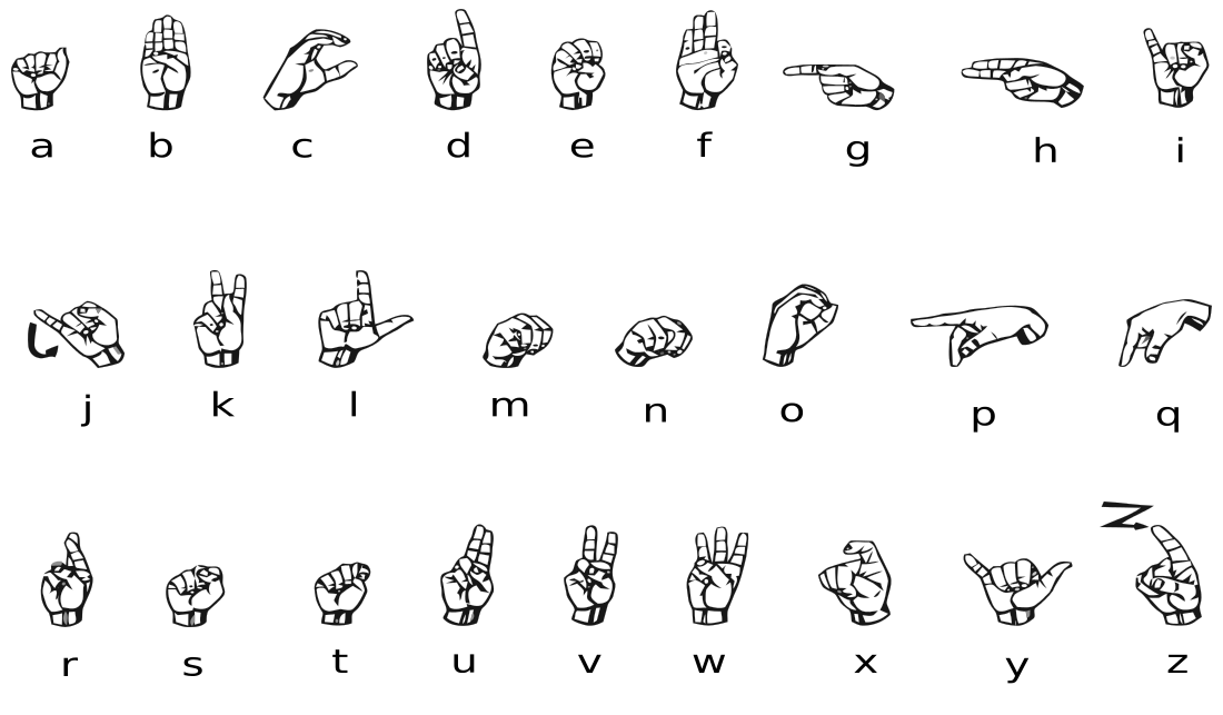
This dataset is available from the website Kaggle, which is a fantastic place to find datasets and other deep learning resources. In addition to providing resources like datasets and "kernels" that are like these notebooks, Kaggle hosts competitions that you can take part in, competing with others in training highly accurate models.

If you're looking to practice or see examples of many deep learning projects, Kaggle is a great site to visit.

Loading the Data

The sign language dataset is in CSV (Comma Separated Values) format, the same data structure behind Microsoft Excel and Google Sheets. It is a grid of rows and columns with labels at the top, as seen in the train and valid datasets (they may take a moment to load).

To load and work with the data, we'll be using a library called Pandas, which is a highly performant tool for loading and manipulating data. We'll read the CSV files into a format called a DataFrame.

Build the Model

The data is all prepared, we have normalized images for training and validation, as well as categorically encoded labels for training and validation.

we are going to build a sequential model. build a model that:

Has a dense input layer. This layer should contain 512 neurons, use the relu activation function, and expect input images with a shape of (784,)
Has a second dense layer with 512 neurons which uses the relu activation function
Has a dense output layer with neurons equal to the number of classes, using the softmax activation function

Creating a model variable to store the model. We've imported the Keras Sequental model class and Dense layer class to get you started.

Creating the Convolutional Model

These days, many data scientists start their projects by borrowing model properties from a similar project. Assuming the problem is not totally unique, there's a great chance that people have created models that will perform well which are posted in online repositories like TensorFlow Hub and the NGC Catalog. Today, we'll provide a model that will work well for this problem.

We covered many of the different kinds of layers in the notebook, and we will go over them all here with links to their documentation. When in doubt, read the official documentation (or ask stackoverflow).

Conv2D

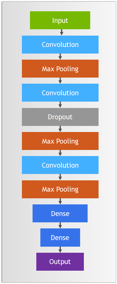
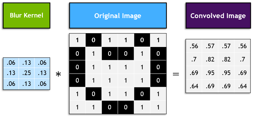
These are our 2D convolutional layers. Small kernels will go over the input image and detect features that are important for classification. Earlier convolutions in the model will detect simple features such as lines. Later convolutions will detect more complex features. Let's look at our first Conv2D layer:

model.add(Conv2D(
                75 , (3,3),
                strides = 1,
                padding = 'same'...)

75 refers to the number of filters that will be learned. (3,3) refers to the size of those filters. Strides refer to the step size that the filter will take as it passes over the image. Padding refers to whether the output image that's created from the filter will match the size of the input image.

BatchNormalization

Like normalizing our inputs, batch normalization scales the values in the hidden layers to improve training. Read more about it in detail here.

MaxPool2D

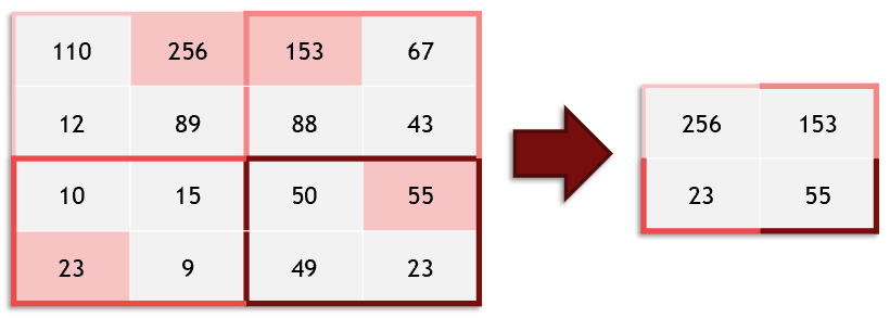
Max pooling takes an image and essentially shrinks it to a lower resolution. It does this to help the model be robust to translation (objects moving side to side), and also makes our model faster.

Dropout

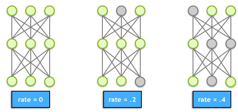
Dropout is a technique for preventing overfitting. Dropout randomly selects a subset of neurons and turns them off, so that they do not participate in forward or backward propagation in that particular pass. This helps to make sure that the network is robust and redundant, and does not rely on any one area to come up with answers.

Flatten

Flatten takes the output of one layer which is multidimensional, and flattens it into a one-dimensional array. The output is called a feature vector and will be connected to the final classification layer.

Dense

We have seen dense layers before in our earlier models. Our first dense layer (512 units) takes the feature vector as input and learns which features will contribute to a particular classification. The second dense layer (24 units) is the final classification layer that outputs our prediction.