 Tracking of the work I did for Xandon's robot which competed in the Seattle Robotics Society's Robo-Magellan event at the Seattle Center on September 20, 2014. This robot ended up placing second in the competition with none of the competitors actually making it to the final cone.
Albert Yen's Clod robot came in first and was able to navigate successfully to one of the bonus cones.
Points of Interest
Newer notes from my 2016 attempt
How to Clone github Repository
Sparkfun 9DoF Sensor Stick Modifications
How to Calibrate the Sparkun 9DoF Sensor Stick
Connected-Component Labeling for Traffic Cone Detection
September 28, 2014
Orientation Sensor - Successful
Overall I think the orientation sensor that I created for this year's Robo-Magellan competition was a success. It appeared to handle well the vibrations, pitching, and rolling that were encountered as the robot maneuvered outside. We only noticed a couple of weaknesses in the final implementation during our testing:
- Ferrous materials and dynamic magnetic fields found in the environment can induce errors into the magnetometer readings. This was however not an issue in the actual competition as the sensor was elevated a bit on the robot. This got it far enough away from the robot's own motors and any other error inducing materials that might have been underground in the competition area.
- Violent shaking will induce errors into the accelerometer readings. The robot used for the competition was too stable to induce such severe vibrations into the sensor so this wasn't a problem.
Currently the code for the orientation sensor is written in Processing/Java and runs on the laptop. One of the first projects I plan to attack for next year's attempt will be to port this code to run on the processor embedded in the orientation sensor itself.
Colour Blob Tracker - Unproven
My colour blob tracker was running on the robot during the competition but wasn't really utilized. This was simply due to the fact that there wasn't enough time to complete all of the necessary navigation code before the day of the competition. Since this code saw very little real world testing outside using the actual camera on the robot, I would say that this code is unproven. However there are a few weaknesses that we do know about from what testing we did accomplish:
- The noise in the data at 640x480 can cause holes in the blobs. Some blob pixels will just fall outside of the expected colour constraints for the traffic cone because of noise alone. There is a downSample constant in my blob sample which can be used to instead run the colour tracker on a bilinear down sampled version of the video frame. This reduces noise since the the colour values of neighbouring pixels are averaged together and the algorithm can run faster since it processes fewer pixels. I found that setting this downSample constant to 5 did help to make the code more robust during my testing.
- The RGB camera on the robot appeared to be very swamped by the IR from the sun on the day of competition. A lot of the cone was actually bright white and the hue/saturation was very washed out. Maybe adding an IR filter or using another camera with better filtering might help in this area.
September 27, 2014
Vision based Traffic Cone Detector
For tracking the orange traffic cones, I wanted a simple colour blob tracker. The goals for my colour blob tracker included:
- Find blobs of contiguous pixels that are close (within specified thresholds) to the known colour of the traffic cone.
- Process pixel colour values as hue, saturation, and brightness (HSB) instead of the more commonly used RGB or YUV as HSB is more reliable across varying light conditions.
- Allow the matching threshold for each of the HSB colour channels to be specified separately so that the colour match can be most specific for hue, a bit less specific for saturation, and even less specific for brightness.
- Return a bounding box for the blob once found in the frame. I chose to use connected-component labeling since it would allow me to return multiple bounding boxes per frame, one for each matching blob found in the frame. It is also an easy algorithm to implement so I knew I could crank it out in a couple of hours.
Connected-Component Labeling
My implementation of the connected-component labeling algorithm can be found here and I will describe its operation in the next section. Wikipedia also has a good description of the core algorithm.
Pseudocode
- The update() method is called for each video frame. The update() method starts out by initializing class members for this frame. The main initialization is on line 123 where an array of Blob pointers, m_pixelLabels, is allocated. There is an entry in this array for each pixel in the frame and they are used to track to which label each pixel belongs. Java will initialize each of these label entries to null. Line 124 also initializes an empty linked list of blobs, m_blobs.
- Note: I will tend to use the terms label and blob interchangeably in this description and the code. A blob is actually a label but with more information such as the bounding box containing the pixels with this label.
- The frame is now processed in two passes:
- The firstPass() walks through each pixel in the frame. It starts in the upper left hand corner, progresses to the right across the top row, moves to the leftmost column of the next row, progresses to the right across this row, and continues this process for each row of the frame. For each pixel it checks to see if it matches the given HSB constraints (ie. does the pixel have a colour close to that of a traffic cone). If it doesn't match then it just continues onto the next pixel but if it does match then it performs the following:
- Calls findNeighbourWithLowestId() to check the pixel's immediate neighbours (via the m_pixelLabels array) to see which ones are already labelled as belonging to a blob. It doesn't need to check all of the neighbours since the ones to its immediate right and below haven't been processed yet. It only needs to process the 4 which have already been encountered (west, north-west, north, and north-east). The findNeighbourWithLowestId() method returns a pointer to the blob with the lowest label id or null if there were no neighbours which already belong to a blob.
- If there is no neighbouring pixel that is already part of a blob then create a new blob, add it to the head of the m_blobs list, initialize that blob's bounding box to just include the current pixel, and finally record this new blob in the m_pixelLabels entry for this pixel.
- If there is a neighbouring pixel then use the current pixel's coordinates to extend the existing blob's bounding box, record the existing blob in the m_pixelLabels entry for this pixel, and then call updateNeighbourEquivalences(). updateNeighbourEquivalences() looks again at each of the neighbouring pixels which are already labelled. For each labeled neighbour that isn't the one with the lowest label id, set its blob equivalent member to the one with the lowest label id. These equivalences will be used in the second pass to coalesce labelled blobs which touch one another.
- Once the first pass is complete, we have a m_blobs linked list of labelled blobs. This list is sorted from highest label id to lowest label id. There are two types of blobs in this list:
- Ones with m_equivalent set to null. These blobs were never found to themselves be in the need of merging with a blob of a lower id. I call these root blobs.
- Ones with m_equivalent not set to null. These blobs need to be merged into a blob with a lower label id.
- The goals of secondPass() are to coalesce all non-root blobs into their equivalent root blob, remove all non-root blobs from the m_blobs list, and complete the information stored for each root blob. To accomplish this it walks the m_blobs linked list in descending label id order, performing the following for each blob:
- If it is a non-root blob then merge it with the blob pointed to by its equivalent member. This merging process just extends the X and Y bounding box limits to include the current blob's bounding box limits.
- If it is a root blob then finalize it by:
- Calculating the final bounding box dimensions (now that the X and Y limits are known.)
- Populating the blob's pixels boolean array with a bit mask of which pixels within the bounding box actually matched the HSB colour constraints.
- Update the m_blobs linked list by pointing the previously encountered root blob's prev pointer to this root blob. This effectively removes all of the non-root blobs which were previously between these two root blobs. Once a non-root blob has been merged into blobs with lower label Ids, they are no longer required.
- The firstPass() walks through each pixel in the frame. It starts in the upper left hand corner, progresses to the right across the top row, moves to the leftmost column of the next row, progresses to the right across this row, and continues this process for each row of the frame. For each pixel it checks to see if it matches the given HSB constraints (ie. does the pixel have a colour close to that of a traffic cone). If it doesn't match then it just continues onto the next pixel but if it does match then it performs the following:
Example
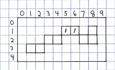
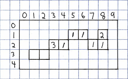
I am now going to manually step through the connected-component labeling algorithm on the following image:
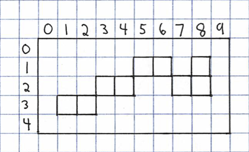
The algorithm starts by looking at the upper left hand pixel (row 0 / column 0). This pixel isn't part of a blob so it will be skipped and it continues onto the pixel to the right. This pixel isn't part of a blob either so it too is skipped. None of the pixels in row 0 belong to a blob so they are all skipped. This skipping continues until we get to the pixel in row 1 / column 5. This is the first pixel encountered that belongs to a blob so it will be given a label of 1.
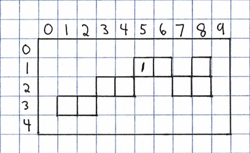
A blob entry will be created with an id of 1 and the X/Y limits set to encompass this pixel in row 1 /column 5.
| Id | Equivalent | minX | minY | maxX | maxY |
|---|---|---|---|---|---|
| 1 | null | 5 | 1 | 5 | 1 |
Now the algorithm progresses to the next pixel at row 1 / column 6. It too belongs to a blob. Looking at the neighbouring pixel to the left it sees that it has a label of 1. The current pixel will be given the same label of 1.
The existing blob entry will have its X/Y limits updated to include this new pixel at row 1 / column 6.
| Id | Equivalent | minX | minY | maxX | maxY |
|---|---|---|---|---|---|
| 1 | null | 5 | 1 | 6 | 1 |
The next pixel to the right doesn't belong to a blob so it will be skipped. The pixel at row 1 / column 8 does belong to a blob. None of the already processed neighbours belong to a blob so it will be given a new label of 2.
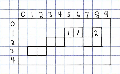
A new blob entry will be added to the head of the list to encompass this latest pixel.
| Id | Equivalent | minX | minY | maxX | maxY |
|---|---|---|---|---|---|
| 2 | null | 8 | 1 | 8 | 1 |
| 1 | null | 5 | 1 | 6 | 1 |
The next pixel encountered that is part of a blob is found at row 2 / column 3. None of its neighbours belong to a blob yet so it will be given a new label of 3.

The blob list now looks like this:
| Id | Equivalent | minX | minY | maxX | maxY |
|---|---|---|---|---|---|
| 3 | null | 3 | 2 | 3 | 2 |
| 2 | null | 8 | 1 | 8 | 1 |
| 1 | null | 5 | 1 | 6 | 1 |
The next pixel at row 2 / column 4 is where things start to get a bit more interesting. It belongs to a blob so it needs a label. When we look at the neighbouring pixels that have already been processed we see that the neighbour to the west has a label of 3 and the one to the north-east has a label of 1. The current pixel will use the id of its lowest neighbour, which is 1 in this case.
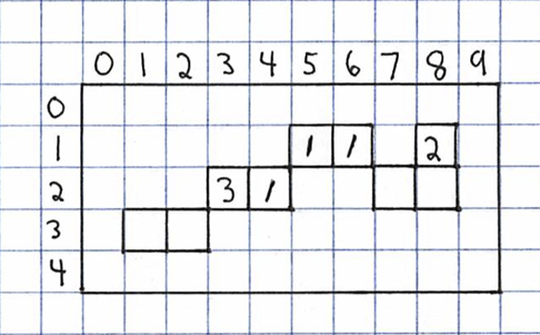
We now know that the blob with a label of 3 is actually part of the blob with a label of 1 so we need to record this equivalency in blob 3's entry. The X/Y limits for blob 1 will also be updated to encompass the new pixel at row 2 / column 4.
| Id | Equivalent | minX | minY | maxX | maxY |
|---|---|---|---|---|---|
| 3 | 1 | 3 | 2 | 3 | 2 |
| 2 | null | 8 | 1 | 8 | 1 |
| 1 | null | 4 | 1 | 6 | 2 |
The next pixel of interest is at row 2 / column 7. It is part of a blob and its north-west neighbour has an id of 1 while its north-east neighbour has an id of 2. This pixel will be given the lowest id of its neighbours, which is 1.
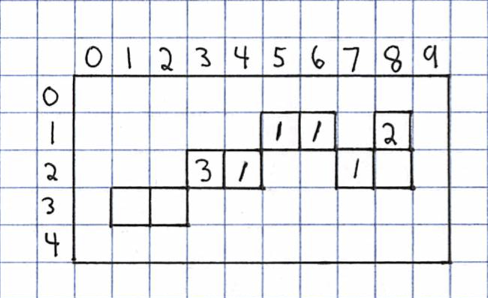
We now know that the blob with a label of 2 is equivalent to the blob with a label of 1. This fact along with including the current pixel's coordinates in the X/Y limits of blob 1 will be recorded in the blob list.
| Id | Equivalent | minX | minY | maxX | maxY |
|---|---|---|---|---|---|
| 3 | 1 | 3 | 2 | 3 | 2 |
| 2 | 1 | 8 | 1 | 8 | 1 |
| 1 | null | 4 | 1 | 7 | 2 |
At the end of row 2, the data structures look like so:
| Id | Equivalent | minX | minY | maxX | maxY |
|---|---|---|---|---|---|
| 3 | 1 | 3 | 2 | 3 | 2 |
| 2 | 1 | 8 | 1 | 8 | 1 |
| 1 | null | 4 | 1 | 8 | 2 |
After all of the rest of the pixels have been processed, the data structures will look like this:
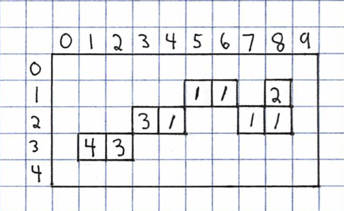
| Id | Equivalent | minX | minY | maxX | maxY |
|---|---|---|---|---|---|
| 4 | 3 | 1 | 3 | 1 | 3 |
| 3 | 1 | 2 | 2 | 3 | 3 |
| 2 | 1 | 8 | 1 | 8 | 1 |
| 1 | null | 4 | 1 | 8 | 2 |
The first pass is now complete. At this point, the algorithm will walk the blob list in descending id order. It merges X/Y limits of the blobs with non-null equivalent values into the equivalent blob and then deletes the non-null entry.
The first entry in the list has a label of 4 and should be merged into blob 3:
| Id | Equivalent | minX | minY | maxX | maxY |
|---|---|---|---|---|---|
| 3 | 1 | 1 | 2 | 3 | 3 |
| 2 | 1 | 8 | 1 | 8 | 1 |
| 1 | null | 4 | 1 | 8 | 2 |
Blob 3 should be merged into blob 1:
| Id | Equivalent | minX | minY | maxX | maxY |
|---|---|---|---|---|---|
| 2 | 1 | 8 | 1 | 8 | 1 |
| 1 | null | 1 | 1 | 8 | 3 |
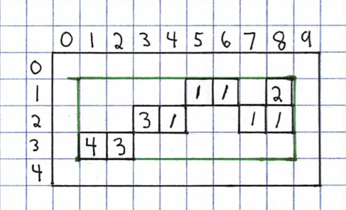
Blob 2 should be merged into blob 1 as well:
| Id | Equivalent | minX | minY | maxX | maxY |
|---|---|---|---|---|---|
| 1 | null | 1 | 1 | 8 | 3 |
At this point we are left with the single blob that we desire. The bounding box starts at (1, 1) and extends to (8, 3).
Processing Colour Blob Tracking Sample
I wrote a Processing based sample for my blob tracking code. This sample can be found at: https://github.com/adamgreen/Ferdinand14/tree/master/blob
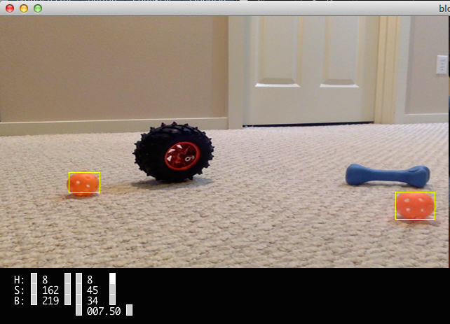
When the application starts, it presents the following UI:
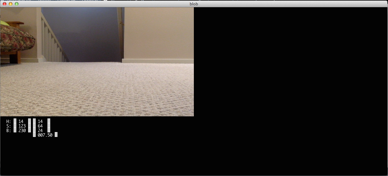
The upper left hand corner shows the live video feed from the selected camera. Below this video feed there are several numbers. Most of these numbers indicate the current hue, saturation, and brightness (HSB) constraints being used by the colour tracking algorithm. The leftmost column of numbers displays the value expected for each colour channel if it is to belong to the blob. The pixel doesn't need to exactly match this value though to be considered a match. The second column displays the variation allowed for each colour channel. When the sample starts it uses the constraints specified in the user's configuration file. In this particular case the values shown in the screenshot above were taken from this configuration data:
blob.camera=name=FaceTime HD Camera,size=640x360,fps=30
blob.hsb=14,123,230
blob.thresholds=14,64,24
blob.minDimension=20
These constraints will consider a pixel to belong to the blob if the colour is within these limits:
| Channel | Range |
|---|---|
| hue | 14 +/- 14 |
| saturation | 123 +/- 64 |
| brightness | 230 +/- 24 |
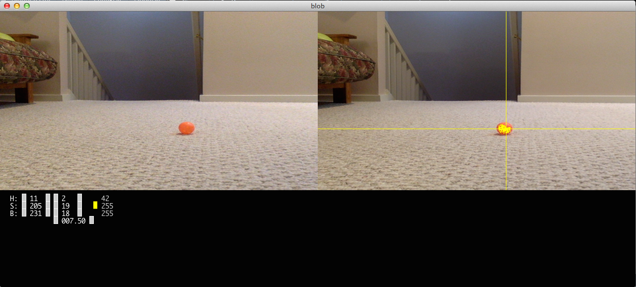
If the user presses the <space> key, the current video frame is copied to the upper right hand part of the window as seen in this screenshot: 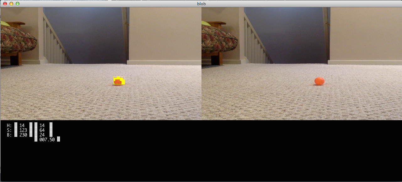
The user can then move the mouse cursor within the captured frame on the right hand side and cross-hairs will be presented to highlight the currently selected pixel. Pressing the mouse button will cause the application to perform a flood fill from the currently selected pixel. The bottom most value in the window (below the HSB thresholds) specifies how closely a pixel must match the colour of its neighbour for it to be used in the flood fill. In these screen shots it was set to the default of 7.50. Setting this to a higher value will loosen the constraints and allow the flood fill to be less specific about the pixels it selects for the fill. The results of the flood fill will be highlighted in the right frame for 2 seconds. In the below screen shot you can see this highlighting. The HSB constraints at the bottom of the window have been updated to cover the minimum and maximum HSB values for the pixels that were filled as part of the flood.
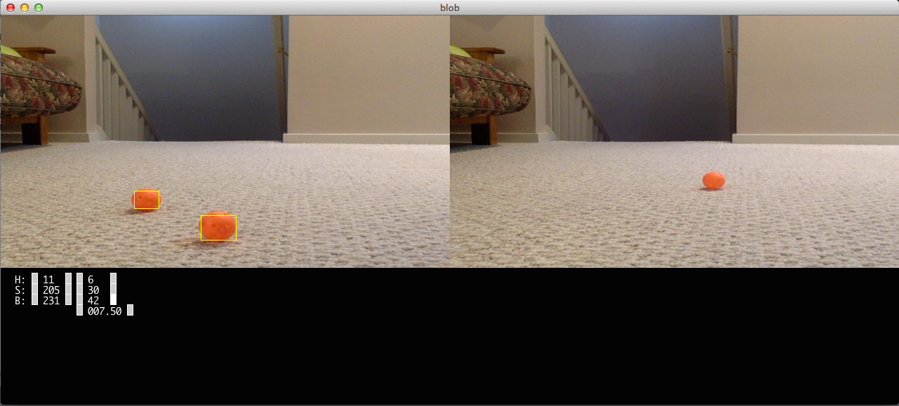
The gray boxes next to the constraint values at the bottom of the window can be used to increase and decrease their associated values. The following screen shot shows the constraints after I modified them by using these keys to make them less restrictive. It also shows the blob tracker successfully tracking two of the orange balls for which it has been configured.
A few other things to note about this sample:
- Pressing the 'H' key will enable/disable the highlighting of the individual pixels which match the constraints. The bounding box will always be drawn.
- When you hover the mouse cursor over pixels in the right frame, additional HSB values will show up in a third column at the bottom of the window. These values represent the HSB values of the currently selected pixel.
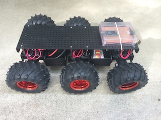
September 24, 2014
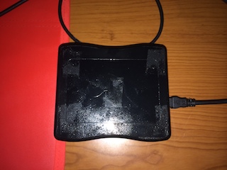
Back in June when I first ordered parts for this Ferdinand2014 project, I also purchased a Wild Thumper 6WD Chassis to use as a test bed. Things got so hectic in the lead up to Robothon 2014 that I didn't get a chance to finish setting it up for computer control until very recently.
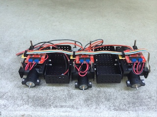
Wild Thumper with Monster Moto Shields
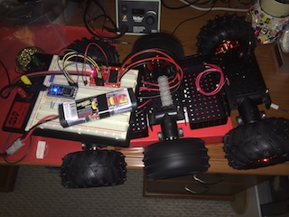
I used a Sparkfun Monster Moto Shield to drive the motors that come with the Wild Thumper chassis. I wrote some very simple code for a mbed LPC1768 micro controller that allows commands to be sent from the PC over a USB based serial connection to control one of these motor shields. That code can be found here. The above photo shows the initial breadboard based prototype for testing of this code. This table gives an overview of how the mbed was wired to the motor controller:
| mbed | Shield | Ribbon Cable |
|---|---|---|
| VU | +5V | 9 - White |
| GND | GND | 10 - Black |
| p21 | d5 - pwm1 | 2 - Red |
| p22 | d6 - pwm2 | 3 - Orange |
| p23 | d7 - ina1 | 4 - Yellow |
| p24 | d8 - inb1 | 5 - Green |
| p25 | d4 - ina2 | 1 - Brown |
| p26 | d9 - inb2 | 6 - Blue |
In the end, I used one Monster Moto Shield for each pair of wheels on the Wild Thumper chassis for a total of three. If all six motors were stalled they could demand more current (3 * 5.5A = 16.5A) than a single motor shield could provide (15A). In the current configuration, the driver chips remain cool to the touch, even if the motors are stalled. If one board was to die this configuration would also allow a quick switch in the field so that a motor could be added to the output of another board. The following two photos show the completed motor wiring with the top plate both removed and installed. The signals from the mbed are fed to all 3 motor shields in parallel so that each motor is commanded to perform the same action.
Wild Thumper Motor Quality
I did my initial testing of the Monster Moto Shields on the center pair of Wild Thumper motors. Once I wired things up such that all six motors would run at the same time, I noticed that these middle motors now run slower and much hotter than the other 4. I think that performing the stall testing on the motor driver with these motors before any kind of break-in might have done some permanent damage to them. Cycling these motors for half hour periods at 3V did seem to make them run a bit better but they still don't perform as well as the rest. I ran the other 4 motors under no load at various voltages (starting at 3V and progressing up to 6V) in an attempt to help break them in more gradually. I will now watch the rest of the motors to see if they develop the same problem or if it is just the early abuse that led to this problem.
September 22, 2014
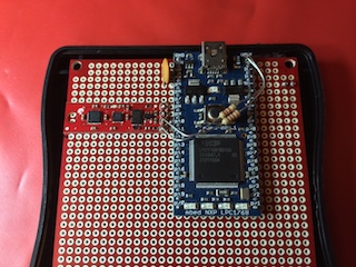
Felix's Brother before Competition
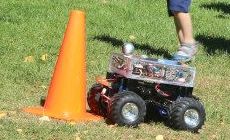
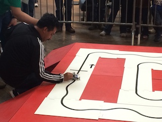
On Saturday evening when I posted some of my photos from that day's Robothon event, I forgot to post the following picture. It shows Xandon's robot as he is preparing it for that day's SRS Robo-Magellan competition.
You can see my orientation sensor mounted on the robot's mast to get it away from the fluctuating magnetic fields caused by the robot's own motors. My orientation sensor was used by the robot's navigation software during the competition and appeared to perform quite well except for one odd heading change that occurred during the final run. I don't know if that was caused by a sudden erroneous output from the orientation sensor or if the higher level code decided to deviate from its current heading for other reasons. Typically the orientation sensor doesn't generate sudden erroneous output when it fails but instead tends to slowly drift towards an incorrect heading. This makes me suspicious that something else occurred in the higher level navigation code.
September 20, 2014
Robothon 2014
Today was Robothon 2014 and I had a great time! I was too busy during the Robo-Magellan competition itself to take any pictures but I did get a few shots of this year's competitors afterwards.

Anthony Witcher and Albert Yen talking shop over Seekeroo.
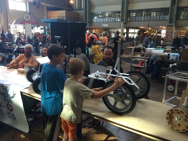
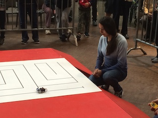
Kids admiring Xandon's robots.
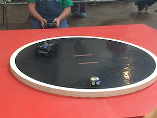
Some of the other Robothon competitions held during the day.
August 19, 2014
Sensor Calibration
In the past I have been kind of random with how I have determined the calibration settings for each of the sensors. To make things easier on myself in the future, I pulled together all of the code I use for calibration into a single application. You can find that application here. An example calibration file that I have created based on this process can be found here.
Magnetometer Calibration
This is one of the easiest and trickiest sensors to calibrate. To calibrate for hard iron distortions we need to obtain the maximum and minimum values that the earth's magnetic field can generate in each axis of the magnetometer. The calibration application can easily track the maximum / minimum readings and display them to the user. The user just needs to manually rotate the orientation sensor so that it encounters each of the maximum/minimum readings. I do this by orienting the device so that each major axis is pointing down and then slowly spiraling it in an ever increasing diameter. The trick is that the hard iron distortion is dependent on the ferrous material located in the immediate vicinity of the magnetometer. That means it should be calibrated when it is actually mounted to the robot so it is the whole robot that needs to be rotated during calibration. The rest of the sensors can be calibrated when detached from the robot. Another trick to keep in mind is that the earth's magnetic field isn't parallel to the surface of the earth but depends on your latitude. Here in Seattle the north vector points downwards with an inclination angle of ~69 degrees. That is the reason I use a spiral motion to find the minimum/maximum readings.
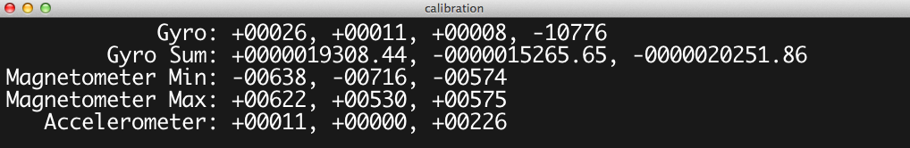
The above screen capture shows the output of the calibration program after I rotated one of my sensors through all of the maximum and minimum orientations. Based on this data, I would place these magnetometer settings in my calibration file:
compass.magnetometer.min=-638,-716,-574
compass.magnetometer.max=622,530,575
Accelerometer Calibration
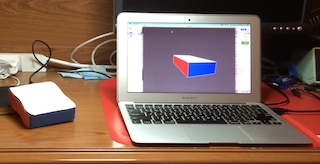
To calibrate the accelerometers we need to obtain the maximum and minimum values that the earth's gravity can generate in each axis. The calibration application shows the current accelerometer readings for each axis. The application only shows the current readings since the minimum and maximum readings would be tainted from accelerations other than gravity as the device is moved. The user can find the minimum and maximum values for each axis by resting the sensor on each of its sides and taking the readings while the device is motionless. You can try placing small shims around the edge of the device while it is laying on its side to make sure that a larger reading can't be found while making sure that the device is level.
The above screen capture shows the output of the calibration program as the orientation sensor lies flat on my desk. It shows that the z accelerometer experiences a maximum reading of 226 when placed in this orientation. Based on this data, I know to set the z field of the compass.accelerometer.max calibration value to 226:
compass.accelerometer.min=-243,-258,-284
compass.accelerometer.max=268,254,226
Laying the device on each of the device's other sides will find the rest of the accelerometer maximum and minimum calibration values.
Gyro Calibration
The gyro will be calibrated in two steps. The first is to determine the relationship between the gyro sensor's temperature and its zero bias (drift) for each axis. The second is to determine the scale of each axis (the number of lsb / degrees per second).
Gyro Drift vs Temperature Calibration
As I mentioned in a previous post, the gyro drift is very dependent on sensor temperature. I start the calibration process by placing the sensor in the freezer for an hour or so to let it cool down.
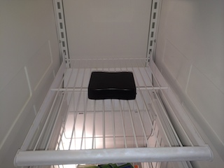
After the hour of cooling, I brought the sensor out to a room temperature location, connected it to my MacBook Air, and started up the calibration application.
As soon as the calibration application starts, it creates a file called gyro.csv. Each minute it logs the average gyro drift measurement along with the temperature. This is an excerpt from the log file it created while one of the orientation sensors was allowed to warm up while also remaining motionless:
temperature,x,y,z
...
-17323.521666666667,9.561166666666667,12.429833333333333,-9.661166666666666
-16635.4485,11.085,12.290166666666666,-7.805
-16061.372166666666,12.331666666666667,12.165333333333333,-6.222
-15552.258166666667,13.721833333333333,12.024833333333333,-4.920833333333333
-15147.791,14.593,11.966666666666667,-3.779166666666667
-14782.6625,15.372166666666667,11.888666666666667,-2.8346666666666667
-14487.181166666667,16.053833333333333,11.851166666666666,-2.0185
-14226.740833333333,16.681,11.7585,-1.3
-13998.222333333333,17.174,11.695666666666666,-0.6775
-13812.186333333333,17.7055,11.583333333333334,-0.14816666666666667
-13605.280833333334,18.079833333333333,11.5405,0.3421666666666667
-13447.805166666667,18.436666666666667,11.469333333333333,0.7943333333333333
-13331.624666666667,18.7685,11.416,1.1536666666666666
-13151.540833333333,19.021333333333335,11.4215,1.5311666666666666
-13075.827666666666,19.420833333333334,11.379166666666666,1.8536666666666666
-12920.863833333333,19.592833333333335,11.3615,2.1441666666666666
-12828.486666666666,19.779833333333332,11.326833333333333,2.4071666666666665
...
I then opened this gyro.csv up in a spreadsheet, graphed the data, and had it calculate a linear equation for a trend line to match the data as well as possible.
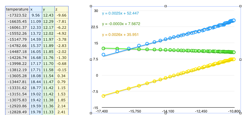
Based on these trend-line equations, I created this calibration data to match the coefficients in the chart:
# These gyro coefficients provide the linear equation (y=ax + b) which relates
# sensor temperature to its bias (drift).
compass.gyro.coefficient.A=0.0025,-0.0003,0.0026
compass.gyro.coefficient.B=52.447,7.5672,35.951
In the future I could have the calibration application calculate the linear least-squares coefficients itself and remove the spreadsheet step.
Gyro Scale Calibration
The best way to calibrate the gyro scale would be to spin the sensor around each axis at a known rotational velocity and take the average of the gyro readings. I don't have a setup here to make such a measurement easy. Instead I accumulate the gyro measurements while rotating the sensor 180 degrees around a particular axis. The second line of the output from the calibration program shows the accumulated readings for each gyro axis. It will be zeroed out when you press the G key. The calibration program also dumps the most recent accumulated results for each axis to the Processing console before it clears the sums.
My calibration process for determining the scale therefore goes something like this:
- Press the G key in the calibration application to clear the gyro measurement sums.
- I watch the gyro sums for a few seconds to make sure that they don't start accumulating readings before I even start to rotate the device. If they do then I jump back to step 1 and try again.
- I then rotate the device 180 degrees about an axis.
- I press the G key again to have the accumulated measurements logged to the Processing console.
- Divide the logged accumulated value by 180 to determine the number of lsb / degrees per second.
I do this process multiple times for each axis and take the average result. These results are then used in the calibration file for this sensor:
# These scale indicates LSBs (least significant bits) per degree.  They should
# be close to the 14.375 value from the ITG-3200 specification.
compass.gyro.scale=14.256,14.021,14.160
August 18, 2014
Orientation Sensor Robustness Issues
While the orientation sensor that I had given to Xandon was working well in static situations, it proved to not be very effective in real world Robo-Magellan scenarios where the robot would be moving and experiencing quite a bit of vibration. The compass heading would be very stable when the robot was stationary but as soon as it started to move the heading could deflect randomly from the true heading, as much as 180 degrees. The simple low-pass filter on the accelerometer and magnetometer measurements alone just wasn't enough to obtain the tilt-compensated compass readings needed for Robo-Magellan navigation. We needed something more!
Gyro Time!
It was at this point that I started looking at the gyro sensors on the Sparkfun 9DoF sensor stick. I saw a great deal of drift in the gyro measurements while the sensor was sitting still, undergoing no rotation. Since the ITG-3200 gyro was the only sensor on the Sparkfun board which also contained a temperature sensor, I decided to write some code which would log this temperature along with the drift error for each axis. Here is a graph of that logged data:
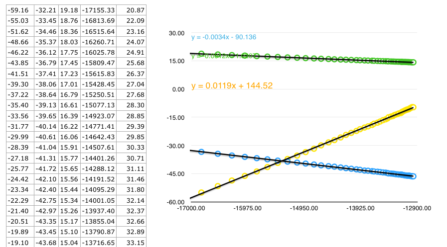
The raw temperature measurements from the sensor are used for the horizontal axis and the raw measurements from each of the gyro axis (x, y, and z) are used for the vertical axis. The sensor was initially placed in the freezer for an hour to cool down the sensor and then moved to a location at room temperature, allowing it to warm up while the logging was taking place. The sensor is stationary while this data was logged so the gyro readings indicate the amount of drift error. The three gyro rotation measurements are in the raw units returned from the sensor (~14.375 lsb / degrees per second.) The temperature is in raw units as well where there are ~280 lsb / C and 35C has a raw value of ~13200. The rightmost field in the table shows the approximate temperature in degrees C [(rawTemp − −13200) ÷ 280 + 35].
It is pretty clear from this graph that there is a linear relationship between the gyro drift and the die temperature. The graph even shows the equation for the first order trend line. I was able to estimate the drift error by using these equation coefficients. Correcting the gyro measurements by subtracting away the estimated drift error resulted in an average drift error of only ~0.5 lsb. The code for performing this correction can be seen here. I will more thoroughly discuss the process I use for calibrating the sensors in a future post.
Kalman Filtering - Finally!
Many on the SRS IRC channel will tell you that I have been talking about solving all of my orientation sensors issues via the magic of Kalman Filters for months now. I would keep suggesting that I would start implementing it tomorrow but once tomorrow came I would be working on another sensor related issue instead. I just kept pushing it out. This all changed on August 14th
commit 6cc50a42c0ccb4cecc1e1adc8dfc5523cf58649a
Author: Adam Green <adamgr@foo.bar>
Date: Thu Aug 14 18:58:41 2014 -0700
Add Kalman filter to gyro Processing sample
This is the initial version of the Kalman filter for fusing the
accelerometer, magnetometer, and gyro sensor measurements together to
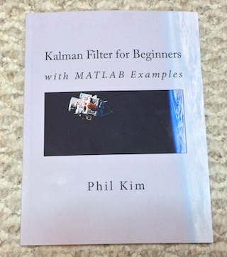
obtain a filtered orientation result.In the end, it didn't take me very long to actually implement this code. It was heavily influenced by Chapter 13. Attitude reference system from the Kalman Filter for Beginners by Phil Kim book.
The Processing code that I am currently using for the Kalman filter can be found in the calculateKalmanRotation() method here.
How well did the Kalman filter work? On August 16th, at the SRS meeting, Xandon integrated the new Kalman version of my code into his Warp project. We then tested it outside on the grass at Renton Technical College. It actually performed much better than I expected! The vibration of driving across the lawn and the swaying motion in the mast of the robot had little influence on the compass heading returned from the orientation sensor. We could drive for a while on the rough terrain and then stop to observe the impact on the orientation sensor. If it had accumulated error then it would have slowly started to correct itself once stopped but that never happened as there was no error for which it needed to correct.
August 17, 2014
It's Been Awhile!
It has been over a month since I last logged any Robo-Magellan progress. I spent a few weeks working on some other projects when I was away from home without access to the orientation sensor. However, I did make some progress on this project and I will cover the highlights in the next few posts:
Lighter MINDS-i Chassis from Carol

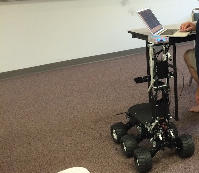
The above photo was taken by Michael Park at Jigsaw Renaissance when Xandon and I met up with Carol to checkout the lighter platform that she had so kindly built us using the MINDS-i Robotics system. It is a very cool platform!! Xandon has been doing some great work over the last month to migrate to the new chassis. In the above photo you can see the RPLIDAR mounted on the front of the new chassis.
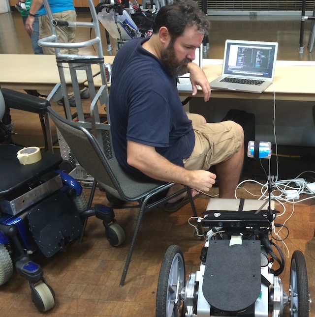
The following photo was taken at the most recent SRS meeting on August 16th while Xandon was integrating and testing my latest orientation sensor code.
July 7, 2014
RoboPeak RPLIDAR Sample in Processing on OS X
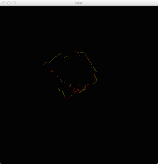
Last Thursday, July 3rd, I worked on creating a Processing port of some C/C++ samples for the RoboPeak RPLIDAR, a low cost 360 degree 2D laser scanner. Xandon received one of these devices a few days ago but there were no existing OS X and/or Processing samples so I thought I would try to solve that problem. I don't actually have one of these devices so I wrote some mbed code to simulate the serial protocol spoken by the RPLIDAR unit and used that for initial testing of my Processing code. I also had a large number of println() statements in the code so that Xandon could run the code with the actual RPLIDAR device and send me the resulting log for debugging purposes.
For the most part, the porting process went pretty smoothly and we really only encountered one hiccup. It turns out that the USB to serial adapter that RoboPeak ships with the unit has the DTR (Data Terminal Ready) output signal connected to the motor enable input on the RPLIDAR unit. I didn't see any mention of this in the documentation so I hadn't done anything special with this signal. When Xandon would run my code, the RPLIDAR would actually stop spinning and not resume to spin until he shutdown my test application. Clearing the DTR signal from my Processing code fixed that issue and then things progressed with no issue. By the early hours of July 4th, we were able to talk to the RPLIDAR unit from OS X and display the 2D scan results on the screen in real time.
Xandon captured a couple of videos of the RPLIDAR which show the output from my Processing sample:
Video of Xandon demoing RPLIDAR sample inside
Video of Xandon demoing RPLIDAR sample outside
The Processing code can be found here: https://github.com/adamgreen/Ferdinand14/blob/master/rplidar/rplidar.pde
The mbed firmware that I used to simulate a RPLIDAR locally can be found here: https://github.com/adamgreen/Ferdinand14/blob/master/rplidar/firmware/main.cpp
July 1, 2014
Happy Canada Day!
Yesterday I modified the orientation sensor firmware to get the sample rate to be exactly 100Hz. The changes I made to the source code to accomplish this include:
- Making the code multithreaded. The sensors are read at 100Hz in a Ticker interrupt handler. The main thread blocks in getSensorReadings() until the next sensor reading becomes available.
- Sampling the ADXL345 accelerometer at 100Hz instead of oversampling at 3200Hz. This uses a lot less CPU cycles, makes it easy to hit 100Hz, and appears to have no impact on the signal to noise ratio.
- No longer having the ADXL345 accelerometer or ITG3200 gyroscope sensor classes wait for the data to be ready before issuing the vector read. The previous code just wasted CPU cycles since the Ticker object is making sure that they are only called at the required 100Hz.
Sparkfun 9DoF Sensor Stick Modifications
I have made two modifications to the Sparkfun 9DoF Sensor Stick to make it work effectively for this project:
- Added a 10uF 0603 SMD tantalum capacitor close to the analog power supply of the ADXL345 accelerometer. Having this extra capacitor decreases the noise I see in the accelerometer readings.
- Switched out the two 4.7k ohm I2C pull-up resistors for stronger 2k ohm resistors. This decreased the rise time of the I2C signals to under 300 nanoseconds as required for reliable 400kHz operation.
I have updated the schematic to show the 9DoF Sensor Stick circuit after my modifications. The following image is an excerpt from the upper-left hand corner of the updated schematic which includes the aforementioned modifications:

For more detailed information about the circuit, you can look at the full schematics:
original schematic from Sparkfun
updated schematic
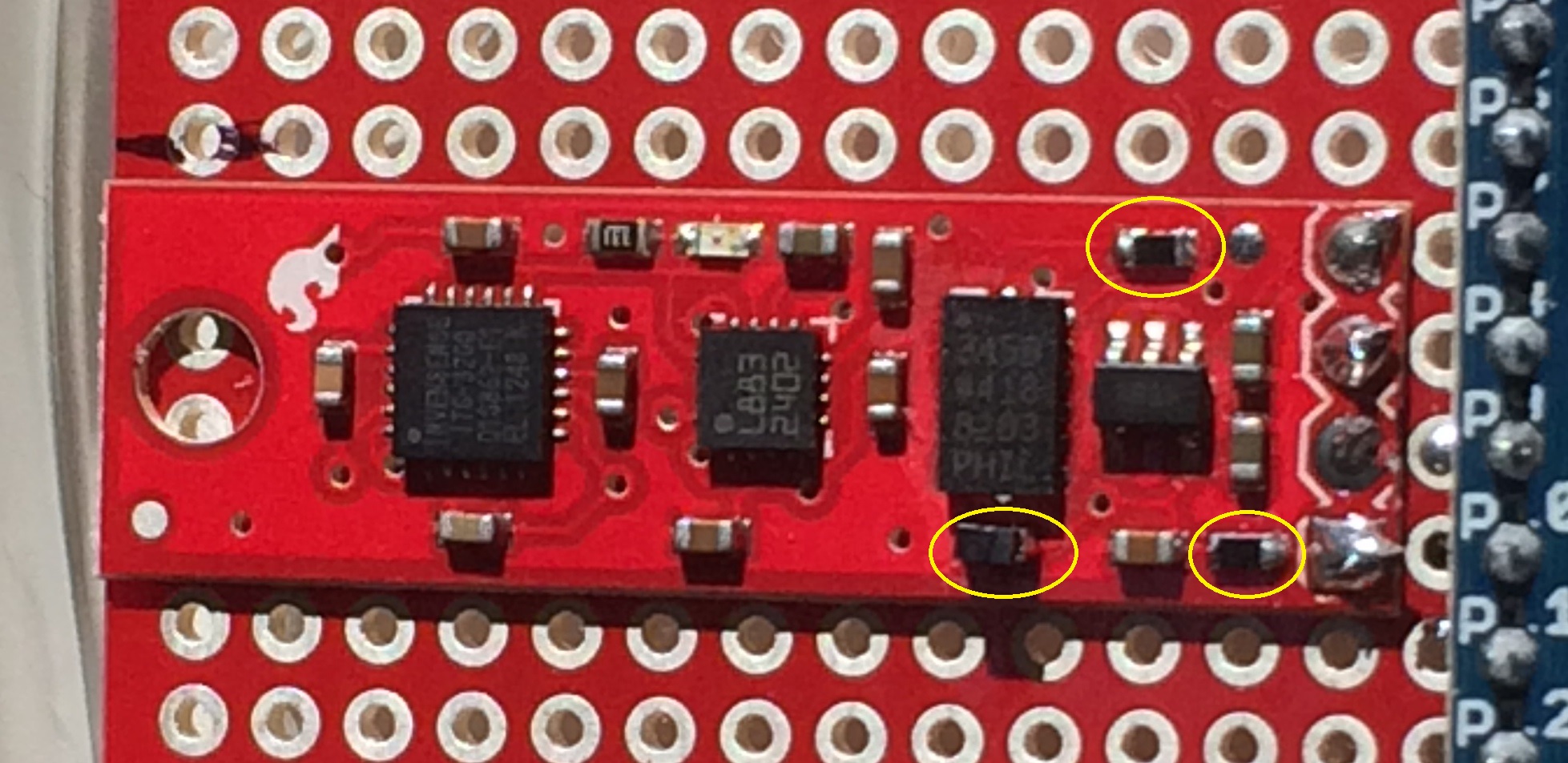
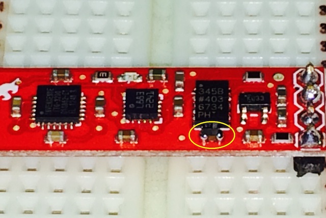
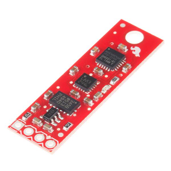
The following image highlights the 3 devices that were updated as part of my modification process:
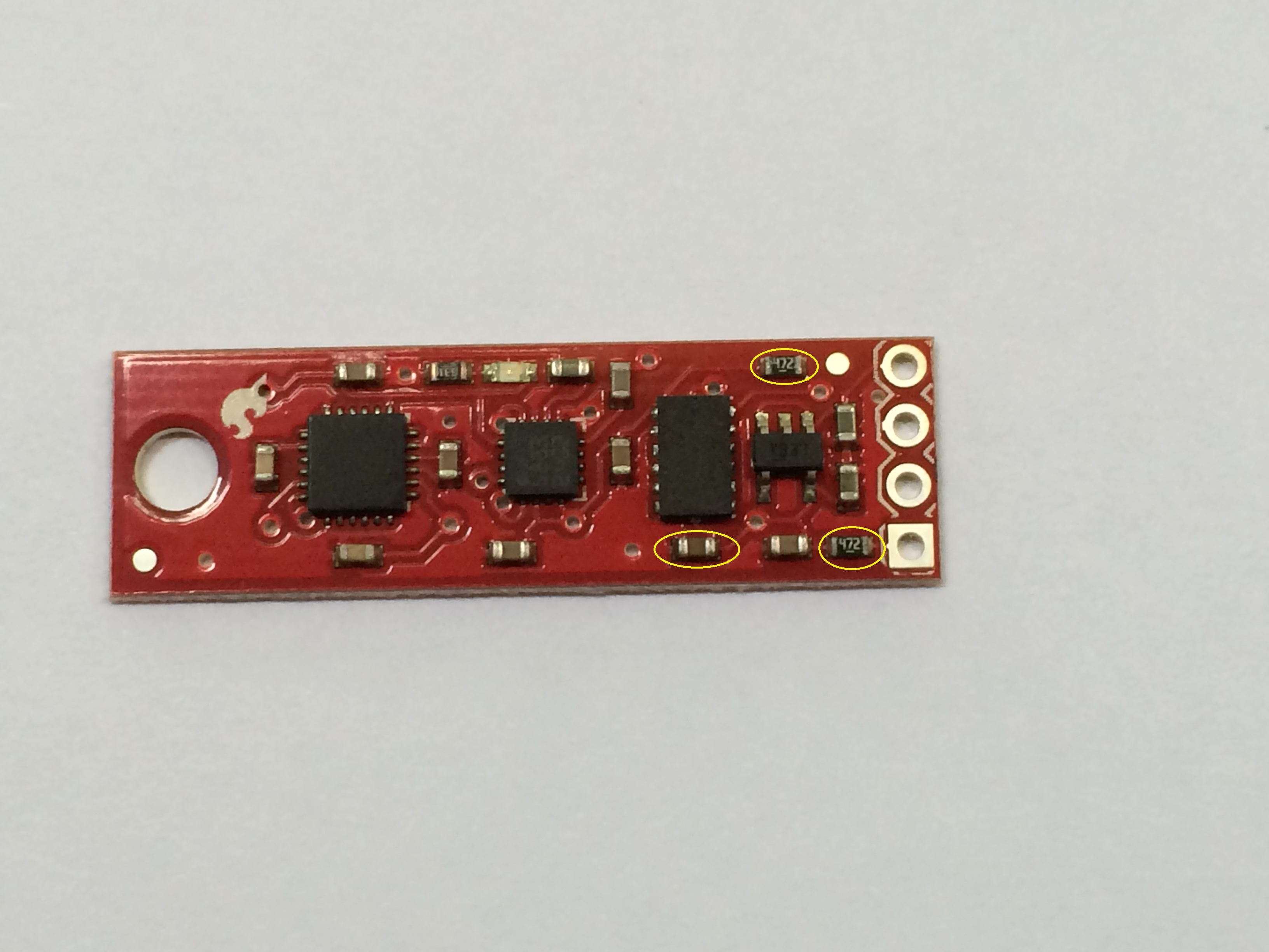
I used my soldering iron to remove the two existing 4.7k ohm resistors (R1 and R2 in the schematic) and then replaced them with 2k ohm resistors of the same 0603 SMD footprint. In the above image, the two resistors replaced were the two highlighted devices labeled as 472.
I soldered a 10uF tantalum capacitor on top of the existing 0.1uF capacitor (C2 in the schematic). This device was polarized so the positive end of the cap (the end with the white band) was placed to the right, the side connected to 3.3V.
The following image highlights the 3 devices after I updated them:
June 30, 2014
While I haven't written anything here for over a week, I have been continuing to make progress on this project:
- I demoed the orientation sensor at the June 21st Seattle Robotics Society, SRS, meeting.
- At the same SRS meeting I handed the first orientation sensor prototype off to Xandon. We also took it outside with his Felix robot to make sure that there was no major interference that would make it completely useless.
- I constructed a second orientation sensor prototype for my own use.
- Met with Xandon again on June 25th to come up with a plan for future testing and feature implementation.
- I updated the compass sample:
- It now reads options like serial port name and calibration settings from a text based configuration file. This allows Xandon and me to both use the same code on our machines even though our hardware configuration is a bit different. An example can be seen here.
- The math for calculating heading and configuring the orientation sensor has been moved into a FilteredCompass class.
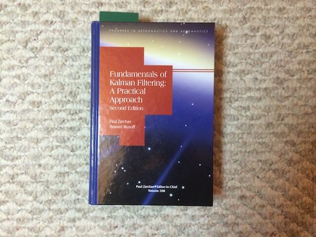
- I continue to make progress reading Fundamentals of Kalman Filtering: A Practical Approach by Paul Zarchan and Howard Musoff
- I updated the firmware to increase the sample rate from 55 to 88 Hz. I plan to make more updates in the future in an attempt to get the sample rate up to 100 Hz.
June 19, 2014
Tonight, I removed the two ugly 2.2k ohm through-hole resistors that can be seen in the June 17th notes. Instead of using these external resistors, I removed the 4.7k ohm SMD resistors from the 9DoF sensor board and replaced them with 0603 2k ohm SMD resistors.
Yesterday, my copy of Kalman Filter for Beginners by Phil Kim arrived from Amazon. I read the whole book last night. It provides a great introduction to Kalman filtering without excessive math. There are even attitude reference examples that are very relevant to the orientation sensor that I am currently working on. I only have two minor complaints about the book: it was translated from Korean to English by a non-native English speaker; and I would have liked to see more discussion on how to troubleshoot the filter when it doesn't work as expected. I plan to adapt the example from Chapter 13, "Attitude reference system" to my orientation sensor project over the next couple of days. I might even have it ready for demoing at the SRS meeting on June 21st.
June 17, 2014
It has been a few days since I updated these notes but I have been making progress on the orientation sensor since the last update.
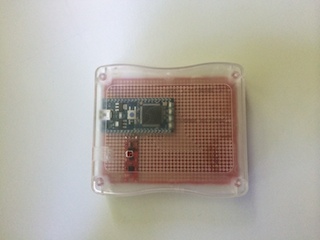
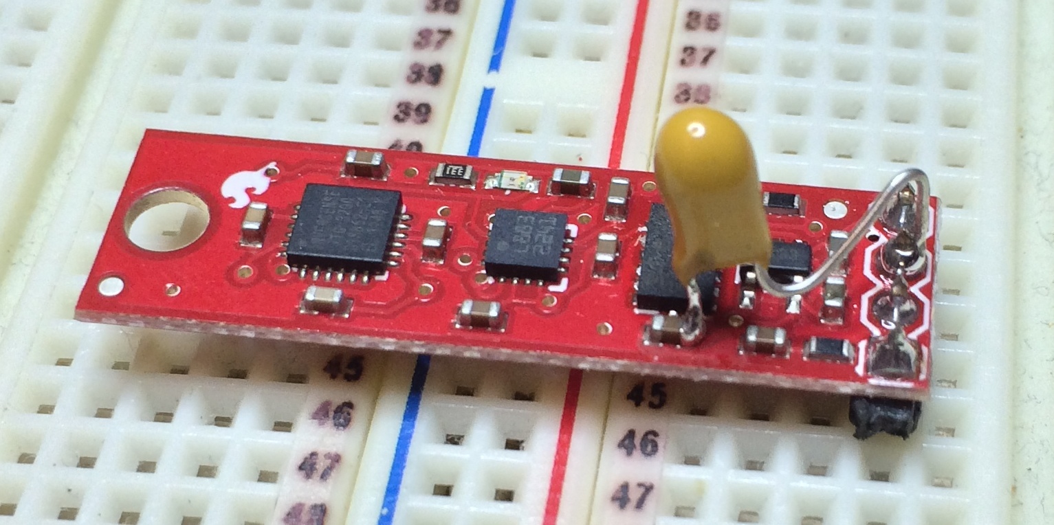
Soldered Prototype
I have moved the Sparkfun 9DoF Sensor Stick and mbed-LPC1768 from the solder-less breadboard and moved it to a more permanent soldered prototyping board to be mounted in a Sparkfun Project Case. The 2.2k ohm resistors in the above image were temporarily soldered on to decrease I2C signal rise times. I have SMD resistors arriving this week that I will just solder onto the 9 DoF board and then remove these temporaries.
Code Updates
I have also made several updates to the code over the last couple of days:
- I refactored the firmware on the mbed:
- Removed redundant code that was copy/pasted into the ADXL345 accelerometer, HMC5883L magnetometer, and ITG3200 gyro classes. The shared code is now found in the SensorBase class from which the other sensor classes derive.
- I also added a Sparkfun9DoFSensorStick class. This class encapsulates the three sensor classes (ADXL345, HMC5883L, and ITG3200) and the main code now just instantiates and queries it for all of the sensor readings.
- Created a template based version of IntVector<> to replace Int16Vector and Int32Vector.
- Now that I have the electronics in a more permanent enclosure, I updated the samples accordingly:
- I updated the magnetometer calibration settings since the hard-iron distortions changed during the move from the solder-less breadboard.
- I added the ability in the Orientation sample to press the <space> bar to have the camera rotated around to face the current location of the front of the device. By default it starts up facing towards the east. Now it can be moved to match the direction the audience is facing.
- I also added coloured paper to the actual prototype enclosure and matched the colours in the virtual device rendered in the Orientation sample. This makes it easier for people viewing the demo to see how what is on the screen matches the orientation of the physical device.
June 13, 2014
Through Hole Out and SMD In
I removed my previous through hole 10uF tantalum bypass capacitor
and replaced it with the 0603 SMD 10uF tantalum capacitor that I received from Digikey today
InvenSense ITG-3200 Gyroscope
Today I added code to my mbed firmware to support reading of the InvenSense ITG-3200 gyroscope sensor and sending the values read back to the PC. The output from this sensor has a bit of zero bias but it doesn't vary by more than +/- 1 LSB when the device is stationary. The only modification I made to the Processing samples so far is to have them accept and ignore the last 3 comma separated gyro values on each line.
Overall I like this sensor board from Sparkfun but I do wish that the accelerometer worked a bit better. I ordered up a second 9DoF board from Sparkfun today so that Xandon and I can run experiments with the same hardware. I now need to migrate the hardware from the current breadboard setup to a PCB and then I can concentrate all of my efforts on the filtering software.
June 12, 2014
I spent some time yesterday trying to figure out how I could fix the ADXL345 accelerometer noise. I had originally thought that oversampling the accelerometer by reading 32 samples for every 1 of the magnetometer samples (accelerometer sampled at 3200Hz and magnetometer sampled at 100Hz) and just using the average of those 32 samples would be enough but that resulted in the same amount of wild fluctuation in the readings. When I attached the oscilloscope as close to the analog supply line as possible, I saw ripple at 20kHz but the amplitude of that ripple would vary at a much lower frequency.
I ordered some 10uF tantalum SMD capacitors to gang up with the existing 0.1uF ceramic capacitors already on that supply line but while I was waiting, I found a through hole tantalum and bodged it on instead.
The result is an ugly board but a usable accelerometer. With this hardware fix, the 32x oversampling and a bit more low pass filtering on the PC side, the samples now work much better than they have ever worked in the past.
June 10, 2014
Last night and today were very productive. Last night I was able to get the firmware running on the mbed to properly read the ADXL345 accelerometer and HMC5883L magnetometer to transfer back to the PC over the USB serial connection. Today I updated the Processing samples to work with the new sensor readings. For the most part, this only required two major changes to the existing code:
- Updating the accelerometer and magnetometer calibration settings in all of the samples:
- These calibration values provide the minimum and maximum readings obtained from the sensors when detecting gravity and the earth's magnetic field.
- This calibration data is then used to adjust the zero point for each sensor axis (ie. it is not always the case that a zero reading from a sensor corresponds to a real world zero value since there is often an error bias in the sensors.)
- Also appropriately scales the readings for each sensor:
- Scales the minimum and maximum accelerometer values to represent -1.0g and 1.0g.
- Scales each of the magnetometer axis to remove any elliptic hard iron distortions.
- Permuting the X, Y, and Z values as required. This is required for two reasons:
- The X, Y, and Z axis of the sensors don't necessarily line up with the X, Y, and Z axis used for rendering 3D objects in Processing samples such as Orientation.pde.
- Each of the 3 sensors included on the Sparkfun 9DoF board are arranged with their axis pointing in different directions.
Good News
The HMC5883L magnetometer data output is much cleaner than what I previously obtained from the LSM303DLH. The fact that the sensor itself can be configured to average together 8 samples per reading helps a lot in this area.
Bad News
The ADXL345 accelerometer data output is much noisier than the LSM303DLH. This on top of the fact that it isn't as sensitive (the LSM303DLH is 950 - 1055 LSB/g and the ADXL345 is only 256 LSB/g) makes the 3D orientation data much more shaky.
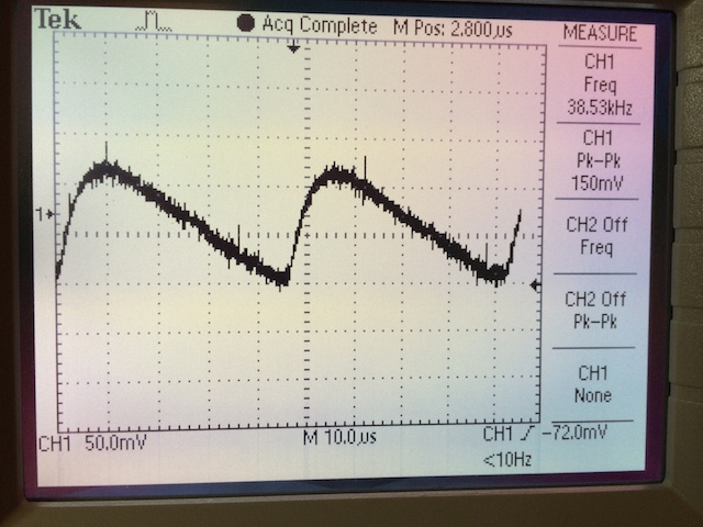
I2C Signals
I figured before I cranked the I2C rate up to 400kHz from 100kHz, I should take a look at the rise times of the SCL and SDA lines with the oscilloscope. When I scoped the SCL line what did I see? This!
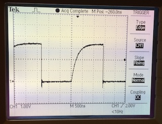
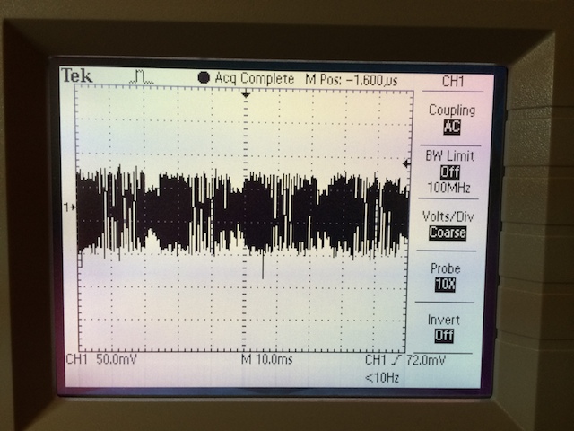
This rise time looks a lot worse than the 300 nsec requirement I see in the sensor data sheets. It would appear that the 4.7k ohm pull-up resistors installed by Sparkfun might be a bit much. I added some 2.2k ohm resistors in parallel to see what the resulting signal would look like:

I think I will leave those extra resistors there!
June 9, 2014
Clone this Repo and its Submodules
Today, as I got started on porting the firmware to utilize the new sensors, I noticed that I hadn't made the GCC4MBED dependency explicit in the Ferdinand2014 project. To remedy this problem, I have added it as a submodule.
Cloning now requires a few more options to fetch all of the necessary code.
git clone --recursive git@github.com:adamgreen/Ferdinand14.git
- In the gcc4mbed subdirectory you will find multiple install scripts. Run the install script appropriate for your platform:
- Windows: win_install.cmd
- OS X: mac_install
- Linux: linux_install
- You can then run the BuildShell script which will be created during the install to properly configure the PATH environment variable. You may want to edit this script to further customize your development environment.
Important Notes:
- OS X Mountain Lion and newer will fail to execute mac_install by simply clicking on it. Instead right click on mac_install in the Finder, select the Open option, and then click the Open button in the resulting security warning dialog.
- If the installation should fail, please refer to win_install.log, linux_install.log, or mac_install.log. It will contain the details of the installation process and any errors that were encountered.
Wiring up the Sparkfun 9 Degrees of Freedom - Sensor Stick

I now have the 4-pin male header soldered onto the Sparkfun 9 DoF Sensor Stick and it now replaces the older LSM303DLH sensor breakout board that I was previously using on my breadboard. There aren't a lot of wires to connect for this sensor:
| 9DoF Sensor Stick | mbed Pin |
|---|---|
| Vcc | p40 - VU (5.0v USB Out) |
| Gnd | p1 - GND |
| SDA | p9 - I2C SDA |
| SCL | p10 - I2C SCL |
Nothing left to do now except for starting to write some code. Yippee!
Porting Firmware
Tonight, I started porting the firmware running on the mbed 1768 to use the ADXL345 accelerometer and HMC5883L magnetometer instead of the older LSM303DLH device. I was able to get it working with the new sensors in a few hours. It nows reads the sensors and sends the readings to the PC over the USB based serial port as comma separated text values. This is an example of a few lines captured during a recent debug run:
15,7,229,-184,-139,-661
20,4,226,-186,-139,-661
20,6,237,-186,-138,-661
16,5,237,-187,-137,-662
My initial look at the data would appear to indicate that the magnetometer data is probably a bit cleaner than the previous sensor. The internal averaging of 8 samples per data read probably helps a lot. There does however appear to be a great deal of noise on the accelerometer readings. The ADXL345 sensors were already 4x less sensitive than the ones in the LSM303DLH device so the extra noise only makes things worse.
I suspect that a good proportion of the accelerometer noise comes from flaws in the Sparkfun 9DoF board design itself. It uses a single supply for both the analog and digital domain. This was not recommended by Analog Devices in the ADXL345 data sheet and if it was to be done, it recommended a lot more filtering to be used than what Sparkfun used. I can think of a few solutions:
- Add capacitors to the analog supply on the ADXL345 as recommended in the data sheet.
- Place a ferrite bead in series with the analog supply as also recommended by the data sheet.
- Use software to further filter the data. While the HMC5883L magnetometer can only be sampled at 160Hz maximum, the ADXL345 can be sampled at 3200Hz. One solution would be to oversample the ADXL345 at the full 3200Hz and then average several readings together to present filtered data at the lower rate achievable by the magnetometer.
As I am a software guy, I will try the last solution first :)
Test Platform
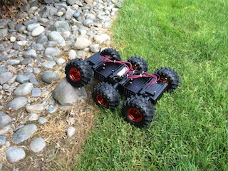
I had also added a Wild Thumper 6WD Chassis to last week's Sparkfun order. I plan to use this for early testing of my sensor prototypes. It is small and light which means that it is easy to transport but it will also bounce around a lot in outdoor environments which is a very good stress test for things like the IMU and camera solutions.
June 8, 2014
Today, I finished reading the data sheets for the Analog Devices ADXL345 accelerometer, Honeywell HMC5883L magnetometer, and InvenSense ITG-3200 gyroscope sensors. Copies of these data sheets can be found here.
Notes:
- Sampling Rates:
- ADXL345: 6.25 - 3200 Hz in multiples of 2x
- ITG-3200: 3.9 - 8000 Hz (maximum filter bandwidth is 256Hz though)
- HMC5883L: 0 - 160 Hz in manual mode
- 100 Hz is a sampling rate common to all 3 devices. It should also be possible to oversample the faster sensors and average them to reduce noise.
- All 3 of the sensors support I2C up to 400 kHz.
- The Sparkfun board only exposes the SDA and SCL data lines along with Vcc and Gnd.
- The board doesn't expose any of the interrupt signals so they can't be used. Need to just rely on the I2C exposed registers.
- The analog and digital supplies are shared across all sensors. This can allow digital ripple onto the analog supply, introducing noise in the analog readings. The ADXL345 data sheet actually recommends more filtering of the analog supply than what is found on the Sparkfun board when a single supply is used like this. I might need to increase the filtering on the board to help reduce noise.
- The self-test feature of the HMC58853L can be used at runtime to compensate for temperature.
- The ITG-3200 has a built in temperature sensor that can be read at the same time as the gyro measurements.
- The Sparkfun board should be mounted close to PCB standoffs to dampen vibrations being coupled into the accelerometer.
- Don't run any current carrying traces under the sensor board, especially the magnetometer.
I2C Addresses as configured on Sparkfun sensor board:
| Sensor | I2C Address |
|---|---|
| ADXL345 | 0x53 |
| HMC5883L | 0x1E |
| ITG-3200 | 0x68 |
At this point, I have enough information to start porting my existing orientation code to use these new sensors. I plan to start on that porting work tomorrow.
June 6, 2014

My Sparkfun order arrived this morning. Within the large red package of electronic goodies was the Sparkfun 9DoF Sensor Stick. I now have almost no excuses to not solder on a header and start porting my orientation code. However I do want to give myself another day or two to try getting my current simulator project finished up before I switch gears and dedicate a substantial amount of time to Robo-Magellan.
June 4, 2014
While waiting for my new Sparkfun 9DoF Sensor Stick to arrive, I am doing a bit of light reading to learn more about Kalman filters. I plan to use Kalman filtering to improve the robustness of my IMU by fusing in the gyro readings with the accelerometer and magnetometer readings that I am already using. This light reading currently consists of pulling this 700+ page Fundamentals of Kalman Filtering: A Practical Approach by Paul Zarchan and Howard Musoff book off of my shelf to start the fun learning process. If you don't see me here again anytime soon, you know what happened to me...my brain exploded :)
June 3, 2014
The rules for the SRS Robo-Magellan competition can be found here. The basic goal of this competition is to have an autonomous robot that can navigate between traffic cones that have been placed around the area just in front of the Seattle Center Armory.
Robothon 2014
Xandon contacted a few of us on the SRS IRC channel last night to see if any of us would like to join him in preparing a robot to compete in this year's competition (almost 4 months away.) Count me in!
Xandon had lent me some sensors after last year's Robothon so that I could play with them to see if I could build a robust heading sensor to help with Robo-Magellan outdoor navigation. Over the past several months I have been able to fuse the accelerometer and magnetometer data from the sensors together to give a pretty accurate 3D orientation measurement when the device is static (ie. not moving.) If we could augment this measurement with readings from gyros as well then I think it would be a very useful sensor package for a Robo-Magellan competitor.
My Top Priority
I think it would be nice if Xandon and I could have the same IMU sensors so that both of us can test and develop code at the same time. One of the sensors that I was currently using isn't available from Pololu anymore. I thought it would make sense to switch to a part that was easy to obtain so that we could all have the same IMU package available to us.
Sparkfun 9 Degrees of Freedom - Sensor Stick
I have decided that I would like to try switching to Sparkfun's 9DoF Sensor Stick which contains:
- ADXL345 accelerometer
- HMC5883L magnetometer
- ITG-3200 MEMS gyro
I ordered one of these devices from Sparkfun this morning and it has already shipped. The FedEx tracking information currently indicates that it should be in my eager little hands by Friday.