This project will explore whether there are any relationships between food access in Philadelphia and socioeconomic factors such as poverty level and vehicle availability. The dataset used in this evaluation comes from OpenDataPhilly.org.
Food retail data was collected for unique Census Block Groups within Philadelphia. Each Block Group represents a certain number of residents within a geographic location.
The main attributes on which I focused my analysis are listed below:
- Total Number of High and Low Produce Supply Stores
- Proportion of High Produce Supply Stores
- Supermarket Access (Y/N): based on 0.5 mile radius
- Percent Poverty: percent of residents that fall below the Federal Poverty Line at the time of collection
- Vehicle Availability
- High Produce Supply Stores (HPSS): Stores that carry a certain amount of fresh fruits and vegetables
- Ex: typical supermarkets
- Low Produce Supply Stores (LPSS): stores that carry little to no fresh fruits or vegetables.
- Ex: gas stations and corner stores
- Percent HPSS: HPSS / (HPSS + LPSS)
-
Is there a difference in vehicle availability between areas that have access to supermarkets and those that do not?
-
Is there a difference in the percentage of high produce supply stores based on poverty classification?
The raw dataset had 1336 entries and 17 columns.
Null Values: There were 13 null values within the raw dataset, 11 of which corresponded to the non-residential areas within Philadelphia. These null values were excluded, as I was interested in the areas with residents.
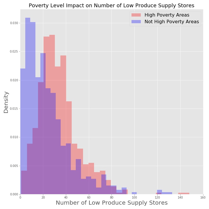
I quickly became interested in the relationship between poverty classification and the number of low produce supply stores. Block Groups were coded "High Poverty" or "Not High Poverty" based on a 20% threshold. It appeared that higher poverty areas could be more likely to have a greater number of low produce supply stores.
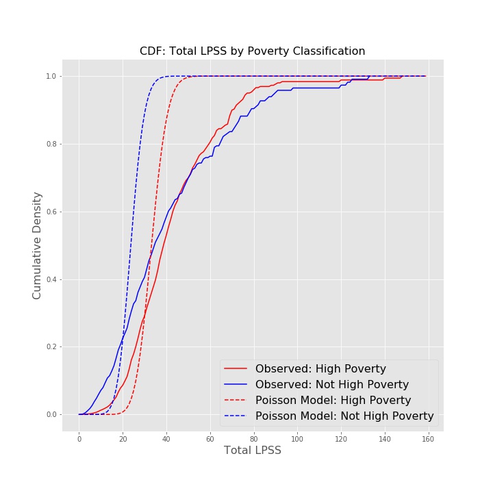
In further exploration, I thought that total LPSS might follow a Poisson distribution, where the unit of space was the Census Block Group and each "event" was the presence of an LPSS. However, the CDFs of the data versus the models clearly show that the data were not generated from a Poisson distribution.
Maximum Likelihood Approach:
- Poisson model to converge on the variable lambda, approximated by the sample means
- Mean(High Poverty Areas) = 33.9 lpss
- Mean(Not High Poverty Areas) = 24.4 lpss
Potential Explanations
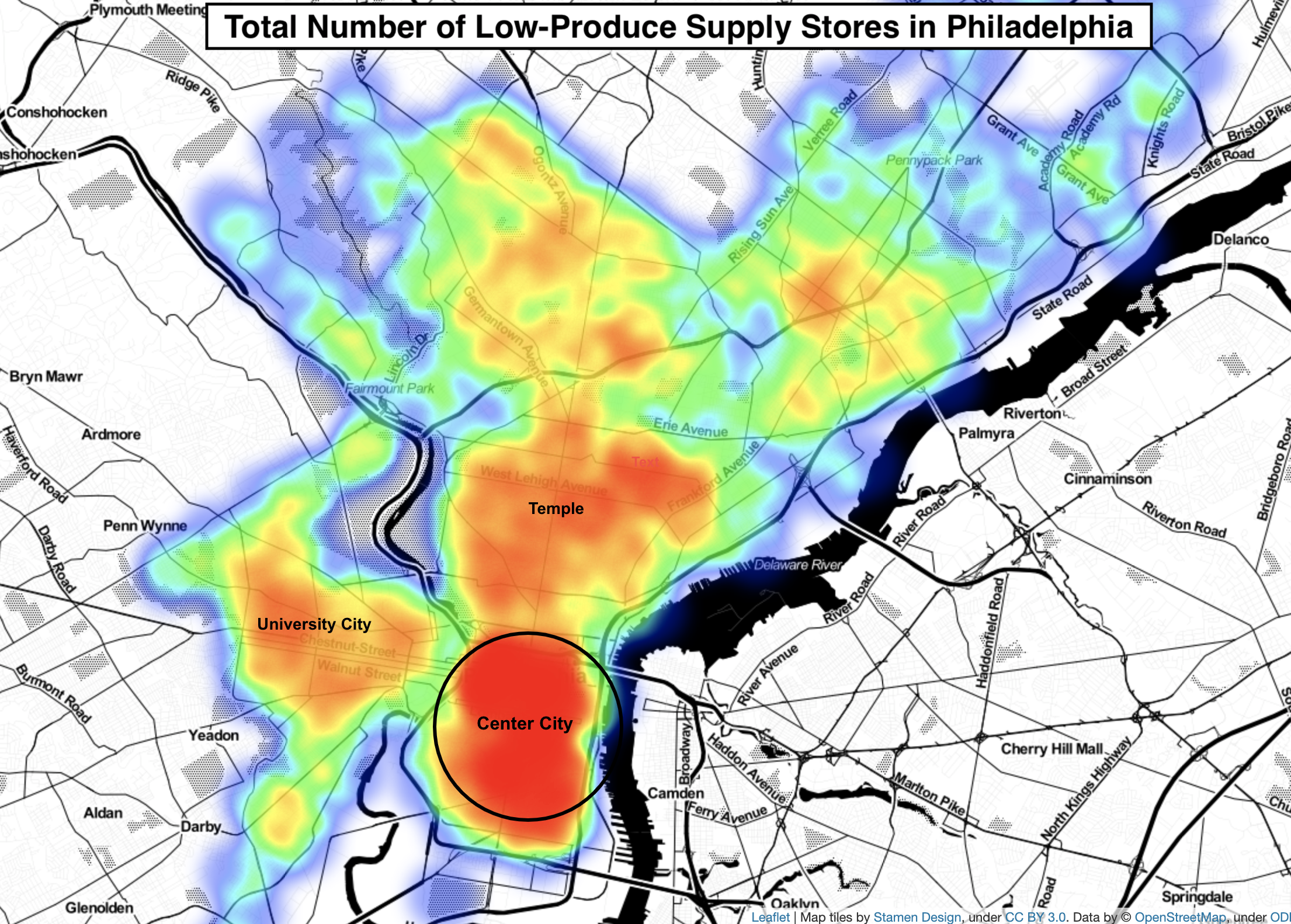
It's likely that our Block Groups are not independent and identically distributed with respect to LPSS; it's more likely that each subsection of Philadlephia has specific demands for the food retail scene. It is interesting that the three areas with the highest number of low produce supply stores are those which likely draw the most non-residents (students and commuters).
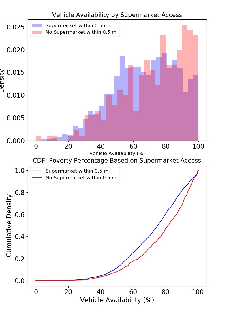
The dataset was split into two categories: Supermarket Access and No Supermarket Access. "Supermarket Access" means that there is a supermarket within 0.5 miles of the Block Group's geolocation. The figures below show distributions for vehicle availability and their observed cumulative densities (CDFs) based on supermarket access. The differences in their CDFs indicate that there may be a difference in vehicle availability between the two groups.
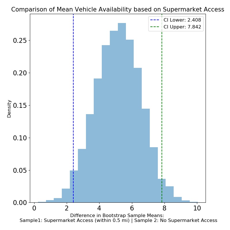
Investigation: Is there a difference in the mean vehicle availability for areas with supermarket access and areas without supermarket access?
Methodology: Comparison of Means
- Relied on boostrapping in order to create a normal distribution of the differences in means between groups (supermarket - no supermarket)
- Number of bootstrap samples = 5,000
- Calculated the 95% confidence interval for the difference in means using the 2.5 and 97.5 percentiles of the distribution of the mean differences
Conclusion: Vehicle availability appears to be higher in areas without supermarket access. We are 95% confident that the difference in mean vehicle availability is between 2.51% and 7.85%.
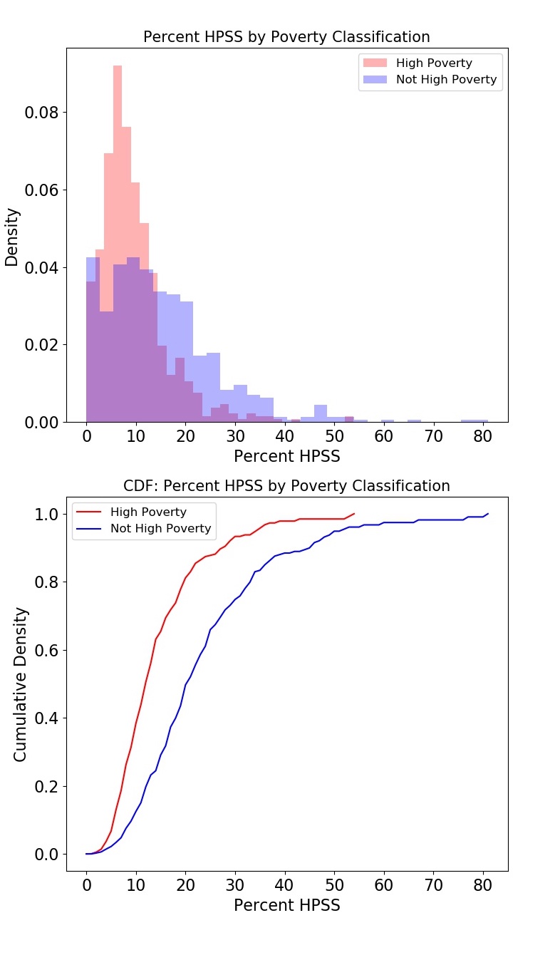
The original dataset was split into two categories: High Poverty and Not High Poverty. High Poverty areas are those in which greater than 20% of residents fall below the Federal Poverty Line. The figures below show the distributions of percent HPSS and the associated cumulative densities for each poverty classification. The differences in their CDFs indicate that not only might there be a difference in mean % HPSS between the two groups, but there could also be a difference in the shape of their distributions.
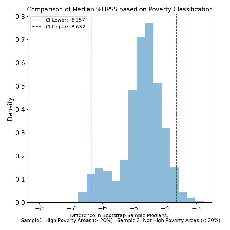
Investigation: Is there a difference in HPSS percentage in High Poverty areas vs. Not High Poverty areas?
Methodology: Comparison of Medians
- Compared medians of the two groups due to right-skewedness
- Relied on boostrapping in order to create a normal distribution of the differences in medians (high poverty - not high poverty)
- Calculated the 95% confidence interval for the difference in medians using the 2.5 and 97.5 percentiles of the distribution of the median differences
Conclusion: Areas with poverty levels above 20% appear to have a lower percentage of HPSS stores than areas with poverty levels below 20%. We are 95% confident that the percentage of HPSS in high poverty areas is between 3.64% and 6.35% lower than non-high poverty areas.
/src/hypo_testing_supermarket.py
/src/hypo_testing_pct_hpss_by_poverty.py
/src/functionalization.py
/notebooks/Exploratory_Data_Analysis.ipynb
-
Dataset: https://www.opendataphilly.org/dataset/showcases/neighborhood-food-retail
-
Technical Appendix: http://foodfitphilly.org/wp-content/uploads/2019/08/Technical-Appendix.pdf
Table 1: Vehicle Availability (%) by Supermarket Access
| Group | Mean | Standard Deviation | n |
|---|---|---|---|
| Supermarket Access | 66.94 | 19.76 | 1051 |
| No Supermarket Access | 72.09 | 20.50 | 272 |
Table 2: HPSS Proportion (%) by Poverty Classification
| Group | Mean | Median | Standard Deviation | n |
|---|---|---|---|---|
| High Poverty | 9.41 | 7.90 | 6.84 | 739 |
| Not High Poverty | 14.87 | 12.5 | 11.53 | 584 |
-
Is there a difference in vehicle access between areas with supermarket access and those without supermarket access?
Null Hypothesis: H0
The mean vehicle availability for areas with supermarket access is the same as the mean vehicle availability for areas without supermarket access (difference in means = 0).
Alternative Hypothesis: HA
The mean vehicle availability in areas with supermarket access is different than the mean vehicle availability in areas without supermarket access (differenc in means != 0).
Significance Level (alpha) = 0.05
Methodology
5,000 bootstrap samples from each group
The the size of each boostrap sample was equal to the number of samples within each group and were chosen at random and with replacement
Calculated the mean of each bootstrap sample and then the difference in means between each group
Calculated 95% confidence intervals as the 2.5 and 97.5 percentiles of the mean differences
-
Is there a difference in the HPSS percentage in High Poverty areas vs. Not High Poverty areas?
Null Hypothesis: H0
The median percent HPSS within high poverty areas is the same as the percent HPSS within areas that are not classified as high poverty (differences in median = 0)
Alternative Hypothesis: HA
The median percent HPSS within high poverty areas is different than the percent HPSS within areas that are not classified as high poverty (differences in median != 0)
Significance Level (alpha) = 0.05
Methodology
5,000 bootstrap samples from each group
The the size of each boostrap sample was equal to the number of samples within each group and were chosen at random and with replacement
Calculated the median of each bootstrap sample and then the difference in medians between each group
Calculated 95% confidence intervals as the 2.5 and 97.5 percentiles of the median differences

