R package for Two-Way Indicator Species Analysis (Hill 1979).
Two-Way Indicator Species Analysis was developed to classify community data tables. It was supposed to work in the same way as a traditional community ecologist in arranging a community data table.
TWINSPAN is available as a self-standing computer program that can be compiled to work on many platforms. This R package uses the same Fortran code, but allows using TWINSPAN from R together with other R functions for community ecology and statistics. The function runs silently – unlike the original TWINSPAN – and most information can be gained analysing the result with support functions provided in this package. Moreover, the package allows using Roleček et al (2009) modification which bases grouping on withing-group heterogeneity instead of cluster level.
You can install the current development version from GitHub using devtools package:
devtools::install_github("jarioksa/twinspan")You need development tools to install a source package. In particular, you need C and Fortran compilers.
If you cannot install a source package, you can install twinspan from R-Universe:
install.packages('twinspan', repos = c('https://jarioksa.r-universe.dev',
'https://cloud.r-project.org'))The basic command to run twinspan is – unsurprisingly – twinspan:
> library(twinspan)
> library(natto) # for data
> data(spurn)
> tw <- twinspan(spurn, cutlevels = 1:6)
The example uses Spurn Point dune scrub data (Shimwell 1971).
TWINSPAN uses basically binary data, and quantitative data are broken into
pseudospecies by species abundances using argument cutlevels. The default cut levels
c(0, 2, 5, 10, 20) are suitable for percentage values, but the spurn data are cover classes.
To keep the original class values, we list all cover classes as cut levels.
The pseudospecies data can be generated with twinsform transformation:
> colnames(twinsform(spurn, cutlevels=0:6))
  [1] "Elaerham1"  "Jacovulg1"  "Soladulc1"  "Rubufrut1"  "UrtidioiA1"
  [6] "Rumecris1"  "ClayperfB1" "StelmediB1" "FestrubrC1" "ElymrepeC1"
... cut ...
 [71] "ElymrepeC3" "AmmoarenC3" "Epilangu3"  "Elaerham4"  "UrtidioiA4"
 [76] "ClayperfB4" "StelmediB4" "FestrubrC4" "ElymrepeC4" "AmmoarenC4"
 [81] "Elaerham5"  "ClayperfB5" "AmmoarenC5" "Elaerham6"
The original data of 40 species are extended to a matrix of 84 pseudospecies.
The names of pseudospecies are formed appending an integer for the cut level
after the species name. Level 1 means that the taxon occurs in the data,
and 6 that it occurs at least the seventh cut level.
The twinspan result can be inspected with support functions of the package.
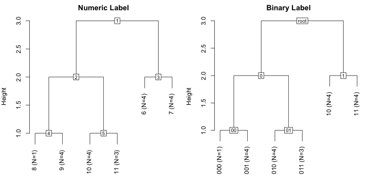
The hierarchy of groups can be displayed as a cluster tree with
> plot(tw, main = "Numeric Label")
> plot(tw, binname = TRUE, main = "Binary Label")
twinspan splits data into two groups and the height of the group shows the
level of hierarchy. The numeric labels are marked within squares, or used
as group names for terminal groups that are no longer divided. The number of
items (N) is also given for each terminal group. When group binname = TRUE), binary text labels are used instead of numbers. The first groups
are 0 and 1, and when these are split 0 or 1 is appended so that the children
of 0 are 00 and 01.
The summary of division process can be inspected with summary (with argument
binname = TRUE binary labels are used instead of numeric):
> summary(tw)
1) eig=0.561:  +ElymrepeC1 < 1
  2) eig=0.4:  -UrtidioiA1 < 0
    4) eig=0.361:  -Soncarve1 < 0
      8) N=1: A19
      9) N=4: A1 A2 A3 A20
    5) eig=0.258:  -ClayperfB4 < 0
      10) N=4: B4 B5 B10 B16
      11) N=3: B12 B17 B18
  3) eig=0.248:  +AmmoarenC4 +Jacovulg1 -Rumecris1 -Soncarve1 < 0
    6) N=4: C6 C8 C9 X14
    7) N=4: C7 C11 C13 C15
twinspan is divisive: it splits data into two parts at each step, and these steps are
described here. The splits are based on the first correspondence analysis axis of the
current subset which is still further polished to make the dichotomy clearer.
twinspan finds the pseudospecies that best indicate the division based on CA axis,
and summary shows these indicator. There are pseudospecies names with + or - signs.
These are used to calculate indicator scores for each quadrat, adding or subtracting
one for each pseudospecies in the quadrat. If the quadrat score is less than the critical
score, we proceed from group ElymrepeC1 (Elymus repens at class value 1). The quadrat score will be 1 for quadrats
with Elymys repens and 0 without, and with condition summary gives the size (N) and lists the names of the member quadrats. Capital letters
A, B, C of the quadrat name give the original classification of Shimwell (1971).
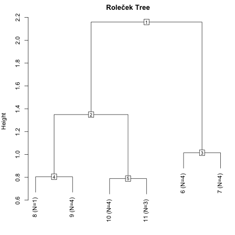
The basic twinspan hierarchy is based on the level of division and it does not
consider within-group heterogeneity. However, the package can evaluate heterogeneities
and use these for trees and further analyses enabling the modification of Roleček et al
(2009):
plot(tw, height = "chi", main = "Roleček Tree")The measure of heterogeneity is the sum of all eigenvalues of group as it is
analysed in twinspan. This is equal to scaled Chi-square, hence the name
"chi" in the argument.
Group 2 of the first-level division is much more heterogeneous than group 3, and for comparable homogeneity of groups it would be best to combine level-1 group 3 with level-2 groups 4 and 5.
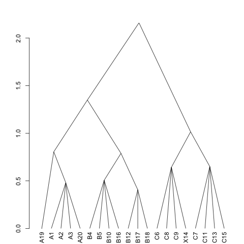
The basic plot and its underlying function as.hclust will use groups as terminal
nodes. With as.dendrogram it is also possible to display quadrats (like they are
called in twinspan):
plot(as.dendrogram(tw, height="chi"), type = "triangle")The dendrogram used the Roleček modification. The first letter of the quadrat name gives the original class (Shimwell 1971), and this is fully recovered with three classes with Roleček modification.
You can extract the classification of each quadrat with cut either for terminal
groups or for a certain level:
> cut(tw)
 [1]  9  9  9 10 10  6  7  6  6 10  7 11  7  6  7 10 11 11  8  9
> cut(tw, level=2)
 [1] 4 4 4 5 5 6 7 6 6 5 7 5 7 6 7 5 5 5 4 4
The Roleček groups respecting heterogeneity can be extracted with cuth ("cut height")
where you must specify the number of groups:
> cuth(tw, ngroups=3)
 [1] 4 4 4 5 5 3 3 3 3 5 3 5 3 3 3 5 5 5 4 4
You can also predict the membership of quadrats based on the indicator pseudospecies
and threshold score. This can also be done with argument newdata using data set that
contains same species, but is not used in developing the classification.
> predict(tw, level=2)
 [1] 4 4 4 5 5 6 7 6 6 5 6 5 7 6 7 5 5 5 4 4
Care is needed with newdata: TWINSPAN will predict a class also when the
newdata is completely unrelated to the original data. If there are no indicator
species, the predicted class will be the one with indicator scores always 0, or group 11
in this example.
TWINSPAN classification is based
on the polished ordination, and the indicator pseudospecies only indicate this
division, and predict based on pseudospecies can give different classificatin than
the actual TWINSPAN that split the data by polished axis of correspondence analysis.
Function misclassified will list the quadrats where the pseudospecies-based and
actual TWINSPAN classification differ. In this simple data set there are no such conflicts.
The data can be tabulated with:
> twintable(tw)

                  00000000000011111111
                  00000111111100001111
                  011110000111

                  A   A  BBBBB   X CCC
                  1AAA2BB11111CCC1C111
                  91230450627868947135
 11111   Bovinigr ---------------1----
 11111   Syntrura -------------1-1----
 11111   Bryuincl ------------1--1----
 11111   Galiveru ------------1--1----
 11111   Ononspin ------------2-------
 11110  BracalbiC ------------1-21-1--
 11101  RanubulbC --------------11-11-
 11101   PoapratC -------------111-211
 11101  ElymrepeC ------------11433111
 11101  FestrubrC ------1-----22121342
 11100   Cladranf ------------------1-
 11100  PlanlancC --------------11-122
 11100  AmmoarenC ------------33115425
 110     Agrostol ----1-----1--111---1
 110     Calysold -------1-1-1-2121--1
 110     Soncarve 1------1----1111-2-1
 10      Verocham 1------1------11----
 01      Rumecris 21111---1--11111-11-
 01      Jacovulg 2212111-1--1--111112
 01      Elaerham 66666666666645353444
 0011    Hypncupr -111--11-------1----
 0011    Epilangu 3---1--112-----1----
 0011    Soladulc 1331211221-11--111--
 00101   Sambnigr ----1---1-----------
 00101   Rubufrut 112-3121111----1----
 001001  Lophhete ----1---------------
 001001 EurhpraeA 22122---------------
 001001  Soncaspe ----1---------------
 001001 UrtidioiA 14223---------------
 001000  Arrhelat 2-------------------
 001000  Hyporadi 1-------------------
 0001    Bracruta --12-1-1-111--------
 0001    Inulcony ----1-----12--------
 000011 CardhirsB ----------11--------
 000011  Heraspho ----------1---------
 000011 CerafontB -------11122--------
 000010 GeasfornB -----11--111--------
 000010 CirsvulgB --------1-1---------
 000010 StelmediB -----2111432--------
 00000  ClayperfB -----4555332--------
20 sites, 40 species
The binary labels before species and above quadrats specify the
grouping. Species names ending in capital letter A, Bor C
where regarded as diagnostic for these quadrat groups
(Shimwell 1971). The table can be large, but you can limit the
number of species or only list "leading species" for each group
(most abundant and frequent in the species group), or species
used as indicators (see summary) or both of these, or you
can subset quadrats.
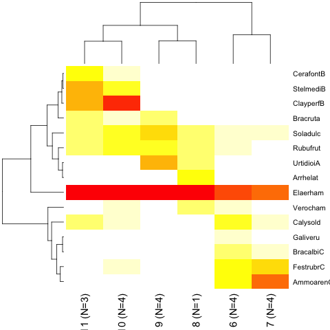
A compact visual summary of classification can be displayed with
> image(tw, height="chi", leadingspecies=TRUE, reorder=TRUE)TWINSPAN stands for TWo-way INdicator SPecies ANalysis, and most of
the functions described above can be used to display species. For instance,
summary(tw, "species") will show the steps of grouping species.
Hill, M.O. (1979) TWINSPAN: A FORTRAN program for arranging multivariate data in an ordered two-way table by classification of the individuals and attributes. Ecology and Systematics, Cornell University, Ithaca, NY.
Roleček, J, Tichý, L., Zelený, D. & Chytrý, M. (2009). Modified TWINSPAN classification in which the hierarchy respects cluster heterogeneity. J Veg Sci 20: 596-602.
Shimwell, D. W. (1971) Description and Classification of Vegetation. Sidgwick & Jackson.


