SAX

S + Autograd + XLA

Autograd and XLA for S-parameters - a scatter parameter circuit simulator and optimizer for the frequency domain based on JAX.

The simulator was developed for simulating Photonic Integrated Circuits but in fact is able to perform any S-parameter based circuit simulation. The goal of SAX is to be a thin wrapper around JAX with some basic tools for S-parameter based circuit simulation and optimization. Therefore, SAX does not define any special datastructures and tries to stay as close as possible to the functional nature of JAX. This makes it very easy to get started with SAX as you only need functions and standard python dictionaries. Let's dive in...

Quick Start

Full Quick Start page - Documentation.

Let's first import the SAX library, along with JAX and the JAX-version of numpy:

import sax
import jax
import jax.numpy as jnp

Define a model function for your component. A SAX model is just a function that returns an 'S-dictionary'. For example a directional coupler:

def coupler(coupling=0.5):
    kappa = coupling**0.5
    tau = (1-coupling)**0.5
    sdict = sax.reciprocal({
        ("in0", "out0"): tau,
        ("in0", "out1"): 1j*kappa,
        ("in1", "out0"): 1j*kappa,
        ("in1", "out1"): tau,
    })
    return sdict

coupler(coupling=0.3)

{('in0', 'out0'): 0.8366600265340756,
 ('in0', 'out1'): 0.5477225575051661j,
 ('in1', 'out0'): 0.5477225575051661j,
 ('in1', 'out1'): 0.8366600265340756,
 ('out0', 'in0'): 0.8366600265340756,
 ('out1', 'in0'): 0.5477225575051661j,
 ('out0', 'in1'): 0.5477225575051661j,
 ('out1', 'in1'): 0.8366600265340756}

Or a waveguide:

def waveguide(wl=1.55, wl0=1.55, neff=2.34, ng=3.4, length=10.0, loss=0.0):
    dwl = wl - wl0
    dneff_dwl = (ng - neff) / wl0
    neff = neff - dwl * dneff_dwl
    phase = 2 * jnp.pi * neff * length / wl
    amplitude = jnp.asarray(10 ** (-loss * length / 20), dtype=complex)
    transmission =  amplitude * jnp.exp(1j * phase)
    sdict = sax.reciprocal({("in0", "out0"): transmission})
    return sdict

waveguide(length=100.0)

{('in0', 'out0'): 0.97953-0.2013j, ('out0', 'in0'): 0.97953-0.2013j}

These component models can then be combined into a circuit:

mzi, _ = sax.circuit(
    netlist={
        "instances": {
            "lft": coupler,
            "top": waveguide,
            "rgt": coupler,
        },
        "connections": {
            "lft,out0": "rgt,in0",
            "lft,out1": "top,in0",
            "top,out0": "rgt,in1",
        },
        "ports": {
            "in0": "lft,in0",
            "in1": "lft,in1",
            "out0": "rgt,out0",
            "out1": "rgt,out1",
        },
    }
)

type(mzi)

function

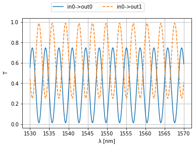
As you can see, the mzi we just created is just another component model function! To simulate it, call the mzi function with the (possibly nested) settings of its subcomponents. Global settings can be added to the 'root' of the circuit call and will be distributed over all subcomponents which have a parameter with the same name (e.g. 'wl'):

wl = jnp.linspace(1.53, 1.57, 1000)
result = mzi(wl=wl, lft={'coupling': 0.3}, top={'length': 200.0}, rgt={'coupling': 0.8})

plt.plot(1e3*wl, jnp.abs(result['in0', 'out0'])**2, label="in0->out0")
plt.plot(1e3*wl, jnp.abs(result['in0', 'out1'])**2, label="in0->out1", ls="--")
plt.xlabel("λ [nm]")
plt.ylabel("T")
plt.grid(True)
plt.figlegend(ncol=2, loc="upper center")
plt.show()

Those are the basics. For more info, check out the full SAX Quick Start page or the rest of the Documentation.

Installation

On Linux, the recommended way to install SAX is as follows:

pip install sax[jax]

On Windows, the recommended way to install SAX is by first setting the PIP_FIND_LINKS environment variable such that the JAX dependency can be installed from a 3rd party repository:

set PIP_FIND_LINKS="https://whls.blob.core.windows.net/unstable/index.html"
pip install sax[jax]

If for whatever reason you don't want the JAX dependency, a JAX-less SAX can also be installed (Note that this is a minimal version of SAX... things might not work as expected. Use on your own risk!):

pip install sax[nojax]

If you want a specific version of JAX, for example if you want a GPU-enabled version of JAX, please read the offical JAX install instructions here.

jaspreetj/sax

SAX

Quick Start

Installation

License