https://blog.miguelgrinberg.com/post/video-streaming-with-flask
- Finding Descriptors (SIFT, SURF, FAST, BRIEF, ORB,BRISK)
- Image Stitching (Brute-Force, FLANN, RANSAC)
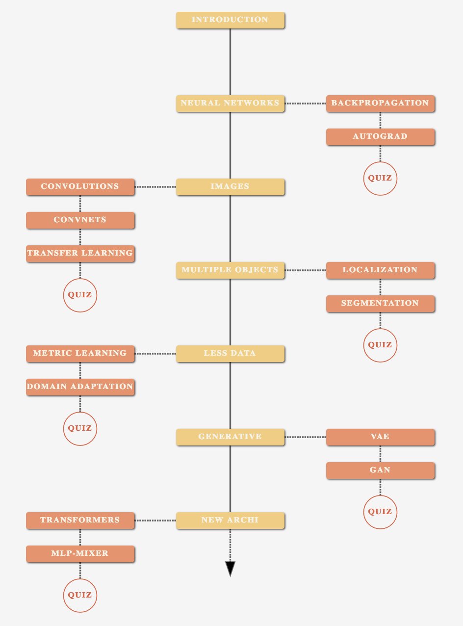
Part 2: Deep Learning (https://arthurdouillard.com/deepcourse/)
- 🧱 Part 1: Basics
- 🎥 Part 2: Video Understing
- 🧭 Part 3: 3D Understing
- SLAM
- 3D reconstruction
- CapsuleNets
- 🖼 Part 4: Generation
- Autoencoder
- GANs
- Part 5: Other
- Super-resolution
- Colourisation
- Style Transfer
- Optical Character Recognition (OCR)
- Part 6: technical
paper = cv2.imread('./Photos/book.jpg')

pts1 = np.float32([ [219,209], [612,8], [380,493], [785,271] ]) # Coordinates that you want to Perspective Transform
pts2 = np.float32([     [0,0], [500,0],   [0,400], [500,400] ])  # Size of the Transformed Image

for val in pt1: cv2.circle(paper,(val[0],val[1]),5,(0,255,0),-1)

# Get transformation matrix M
M = cv2.getPerspectiveTransform(pts1,pts2)          # When manually few (at least 4) points are detceted
#M = cv2.findHomography(pts1,pts2,cv.RANSAC,5.0))   # When lots of matching points, and some of them are errors

dst = cv2.warpPerspective(paper,M,(500,400))
plt.imshow(dst)| SIFT | SURF | FAST | BRIEF | ORB | BRISK | |
|---|---|---|---|---|---|---|
| Year | 1999 | 2006 | 2006 | 2010 | 2011 | 2011 |
| Feature detector | Difference of Gaussian | Fast Hessian | Binary comparison | - | FAST | FAST or AGAST |
| Spectra | Local gradient magnitude | Integral box filter | - | Local binary | Local binary | Local binary |
| Orientation | Yes | Yes | - | No | Yes | Yes |
| Feature shape | Square | HAAR rectangles | - | Square | Square | Square |
| Feature pattern | Square | Dense | - | Random point-par pixel compares | Trained point-par pixel compares | Trained point-par pixel compares |
| Distance func. | Euclidean | Euclidean | - | Hamming | Hamming | Hamming |
| Pros | Accurate | Accurate | FAST (real time) | FAST (real time) | FAST (real time) | FAST (real time) |
| Cons | Slow, patented | Slow, patented | Large number of points | Scale and roation invariant | Less scale invariant | Less scale invariant |
- 3.1 Methods comparison
- Tutorials in openCV
- A Detailed Guide to SIFT for Image Matching (with Python code)
Steps:
- Detecting keypoints (DoG, Harris, etc.) and extracting local invariant descriptors (SIFT, SURF, etc.) from two input images
- Matching the descriptors between the images (overlapping area)
- Using the RANSAC algorithm to estimate a homography matrix using our matched feature vectors
- Applying a warping transformation using the homography matrix obtained from Step #3
- Apply perspective transformation on one image using the other image as a reference frame
- https://www.pyimagesearch.com/2018/12/17/image-stitching-with-opencv-and-python/
- http://datahacker.rs/005-how-to-create-a-panorama-image-using-opencv-with-python/
http://datahacker.rs/013-optical-flow-using-horn-and-schunck-method/
https://arthurdouillard.com/deepcourse/
- Convolutional Neural Network (CNN) For fixed size oredered data, like images
- Variable input size: use adaptative pooling, final layers then:
- Option 1:
AdaptiveAvgPool2d((1, 1))->Linear(num_features, num_classes)(less computation) - Option 2:
Conv2d(num_features, num_classes, 3, padding=1)->AdaptiveAvgPool2d((1, 1))
- Option 1:
- Variable input size: use adaptative pooling, final layers then:
- To speed up jpeg image I/O from the disk one should not use PIL, skimage and even OpenCV but look for libjpeg-turbo or PyVips.
| Description | Paper | |
|---|---|---|
| Inception v3 | Dec 2015 | |
| Resnet | Dec 2015 | |
| SqueezeNet | Feb 2016 | |
| Densenet | Concatenate previous layers | Aug 2016 |
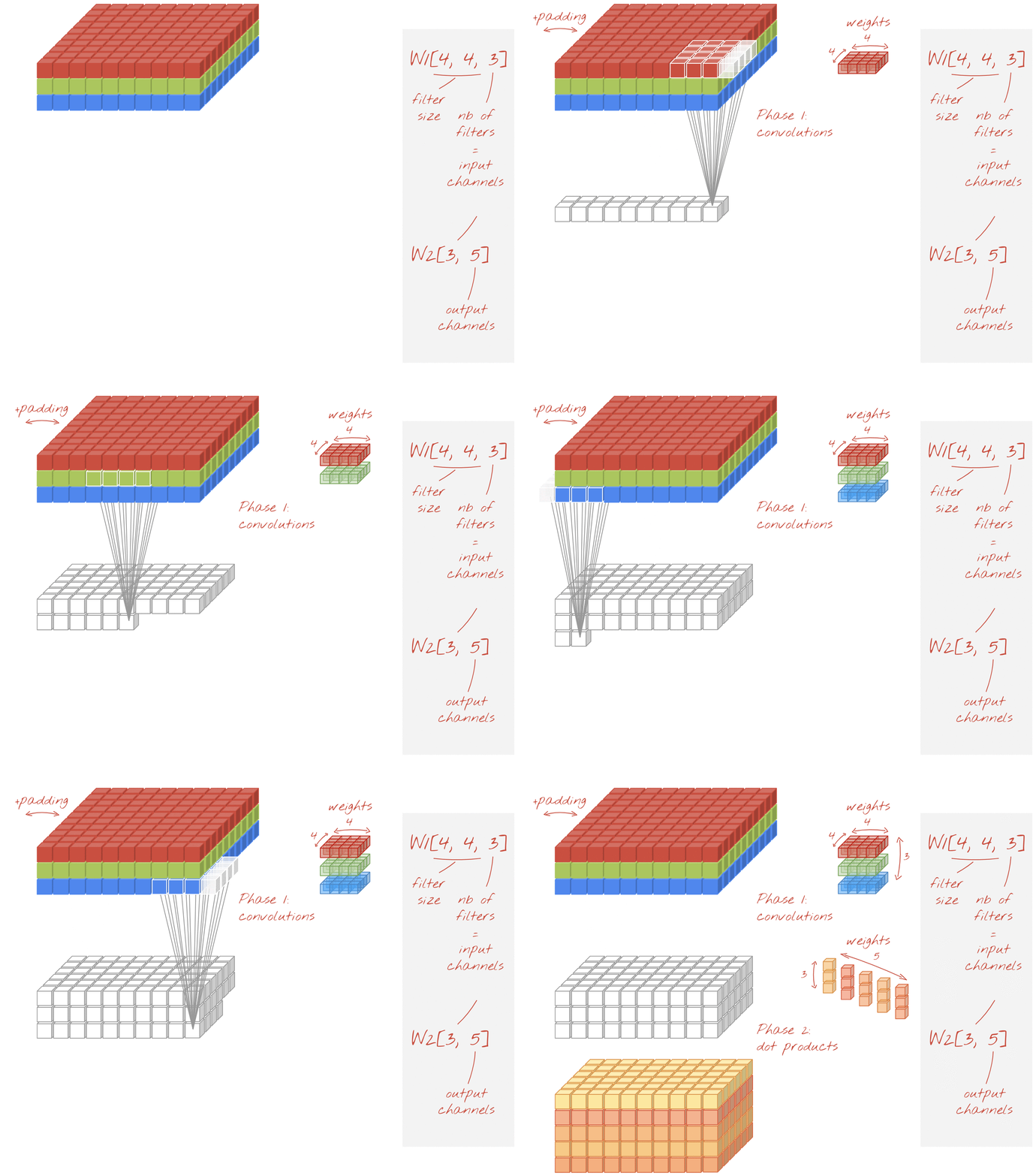
| Xception | Depthwise Separable Convolutions | Oct 2016 |
| ResNext | Nov 2016 | |
| DPN | Dual Path Network | Jul 2017 |
| SENet | Squeeze and Excitation (channels weights) | Sep 2017 |
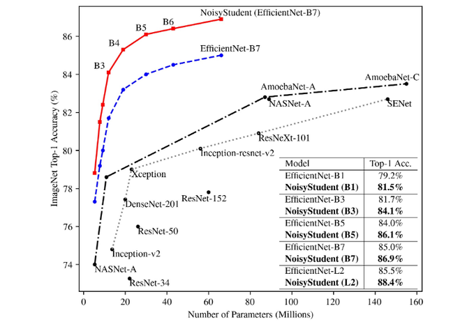
| EfficientNet | Rethinking Model Scaling | May 2019 |
| Noisy Student | Self-training | Nov 2019 |
- Small nets: Useful for mobile phones.
- SqueezeNet (2016): v1.0:
58.108, v1.1:58.250. paper. - Mobilenet v1 (2017):
69.600The standard convolution is decomposed into two. Accuracy similar to Resnet-18. paper - Shufflenet (2017): The most efficient net
67.400. paper. - NASNet-A-Mobile (2017):
74.080. paper - Mobilenet v2 (2018):
71.800. paper - SqueezeNext (2018):
62.640. Hardware-Aware Neural network design. paper.
- SqueezeNet (2016): v1.0:
- Common nets:
- Inception v3 (2015):
77.294paper, blog - Resnet (2015): Every 2 convolutions (3x3->3x3) sum the original input. paper Wide ResNet?
- Resnet-18:
70.142 - Resnet-34:
73.554 - Resnet-50:
76.002. SE-ResNet50:77.636. SE-ResNeXt50 (32x4d):79.076 - Resnet-101:
77.438. SE-ResNet101:78.396. SE-ResNeXt101 (32x4d):80.236 - Resnet-152:
78.428. SE-ResNet152:78.658
- Resnet-18:
- Densenet (2016): Every 2 convolutions (3x3->1x1) concatenate the original input. paper
- DenseNet-121:
74.646 - DenseNet-169:
76.026 - DenseNet-201:
77.152 - DenseNet-161:
77.560
- DenseNet-121:
- Xception (2016):
78.888paper - ResNext (2016): paper
- ResNeXt101 (32x4d):
78.188 - ResNeXt101 (64x4d):
78.956
- ResNeXt101 (32x4d):
- Dual Path Network (DPN): paper
- DualPathNet98:
79.224 - DualPathNet92_5k:
79.400 - DualPathNet131:
79.432 - DualPathNet107_5k:
79.746
- DualPathNet98:
- SENet (2017): Squeeze and Excitation network. Net is allowed to adaptively adjust the weighting of each feature map in the convolution block. paper
- SE-ResNet50:
77.636 - SE-ResNet101:
78.396 - SE-ResNet152:
78.658 - SE-ResNeXt50 (32x4d):
79.076USE THIS ONE FOR A MEDIUM NET - SE-ResNeXt101 (32x4d):
80.236USE THIS ONE FOR A BIG NET
- SE-ResNet50:
- Inception v3 (2015):
- Giants nets: Useful for competitions.
- Features: Average features on the channel axis. This shows all classes detected.
[512, 11, 11]-->[11, 11]. - CAM: Class Activation Map. Final features multiplied by a single class weights and then averaged.
[512, 11, 11]*[512]-->[11, 11]. paper. - Grad-CAM: Final features multiplied by class gradients and the averaged. paper.
- SmoothGrad paper.
- Extra: Distill: feature visualization
- Extra: Distill: building blocks
Get bounding boxes.
Decoding: State Of The Art Object Detection
Check detectron 2.
| Name | Description | Date | Type |
|---|---|---|---|
| R-CNN | Nov 2013 | Region-based | |
| Fast R-CNN | Apr 2015 | Region-based | |
| Faster R-CNN | Jun 2015 | Region-based | |
| YOLO v1 | You Only Look Once | Jun 2015 | Single-shot |
| SSD | Single Shot Detector | Dec 2015 | Single-shot |
| FPN | Feature Pyramid Network | Dec 2016 | Single-shot |
| YOLO v2 | Better, Faster, Stronger | Dec 2016 | Single-shot |
| Mask R-CNN | Mar 2017 | Region-based | |
| RetinaNet | Focal Loss | Aug 2017 | Single-shot |
| PANet | Path Aggregation Network | Mar 2018 | Single-shot |
| YOLO v3 | An Incremental Improvement | Apr 2018 | Single-shot |
| EfficientDet | Based on EfficientNet | Nov 2019 | Single-shot |
| YOLO v4 | Optimal Speed and Accuracy | Apr 2020 | Single-shot |
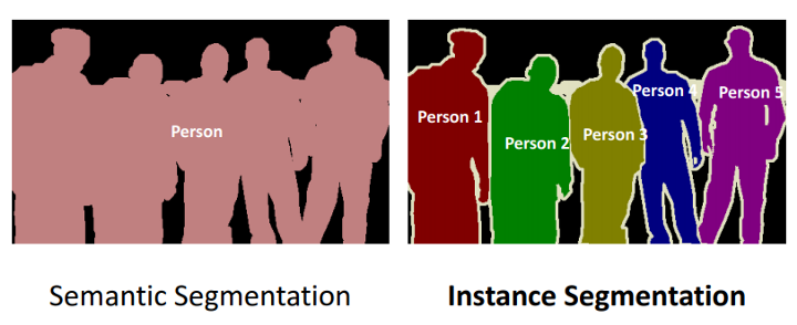
Get pixel-level classes. Note that the model backbone can be a resnet, densenet, inception...
| Name | Description | Date | Instances |
|---|---|---|---|
| FCN | Fully Convolutional Network | 2014 | |
| SegNet | Encoder-decorder | 2015 | |
| Unet | Concatenate like a densenet | 2015 | |
| ENet | Real-time video segmentation | 2016 | |
| PSPNet | Pyramid Scene Parsing Net | 2016 | |
| FPN | Feature Pyramid Networks | 2016 | Yes |
| DeepLabv3 | Increasing dilatation & field-of-view | 2017 | |
| LinkNet | Adds like a resnet | 2017 | |
| PANet | Path Aggregation Network | 2018 | Yes |
| Panop FPN | Panoptic Feature Pyramid Networks | 2019 | ? |
| PointRend | Image Segmentation as Rendering | 2019 | ? |
Feature Pyramid Networks (FPN): slides
Learning the Depths of Moving People by Watching Frozen People (mannequin challenge) paper
- paper (2014)
- Check this kaggle competition
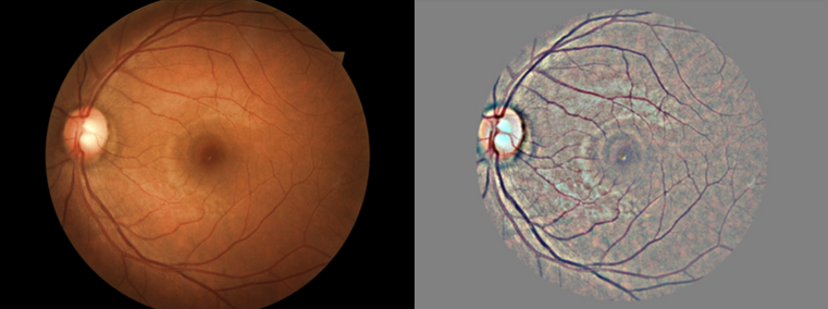
- Fast.ai decrappify & DeOldify
- Image to image problems
- Super Resolution
- Black and white colorization
- Colorful Image Colorization 2016
- DeOldify 2018, SotA
- Decrappification
- Artistic style
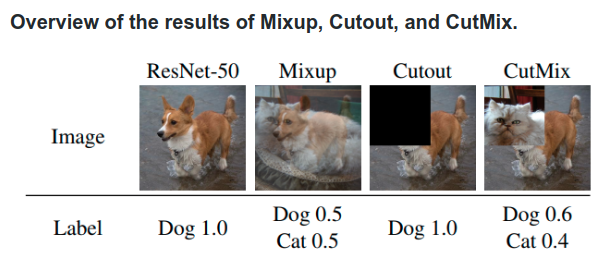
- Data augmentation:
- New images
- From latent vector
- From noise image
- Generate labeled dataset
- Edit ground truth images to become the input images.
- This step depend of the problem: input data could be crappified, black & white, noise, vector ...
- Train the GENERATOR (most of the time)
- Model: UNET with pretrained ResNet backbone + self attention + spectral normalization
- Loss: Mean squared pixel error or L1 loss
- Better Loss: Perceptual Loss (aka Feature Loss)
- Save generated images.
- Train the DISCRIMINATOR (aka Critic) with real vs generated images.
- Model: Pretrained binary classifier + spectral normalization
- Train BOTH nets (ping-pong) with 2 losses (original and discriminator).
- With a NoGAN approach, this step is very quick (a 5% of the total training time, more o less)
- With a traditional progressively-sized GAN approach, this step is very slow.
- If train so much this step, you start seeing artifacts and glitches introduced in renderings.
- Self-Attention GAN (SAGAN): For spatial coherence between regions of the generated image
- Spectral normalization
- Video
- pix2pixHD
- COVST: Naively add temporal consistency.
- Video-to-Video Synthesis
| Paper | Name | Date | Creator |
|---|---|---|---|
| GAN | Generative Adversarial Net | Jun 2014 | Goodfellow |
| CGAN | Conditional GAN | Nov 2014 | Montreal U. |
| DCGAN | Deep Convolutional GAN | Nov 2015 | |
| GAN v2 | Improved GAN | Jun 2016 | Goodfellow |
| InfoGAN | Jun 2016 | OpenAI | |
| CoGAN | Coupled GAN | Jun 2016 | Mitsubishi |
| Pix2Pix | Image to Image | Nov 2016 | Berkeley |
| StackGAN | Text to Image | Dec 2016 | Baidu |
| WGAN | Wasserstein GAN | Jan 2017 | |
| CycleGAN | Cycle GAN | Mar 2017 | Berkeley |
| ProGAN | Progressive growing of GAN | Oct 2017 | NVIDIA |
| SAGAN | Self-Attention GAN | May 2018 | Goodfellow |
| BigGAN | Large Scale GAN Training | Sep 2018 | |
| StyleGAN | Style-based GAN | Dec 2018 | NVIDIA |
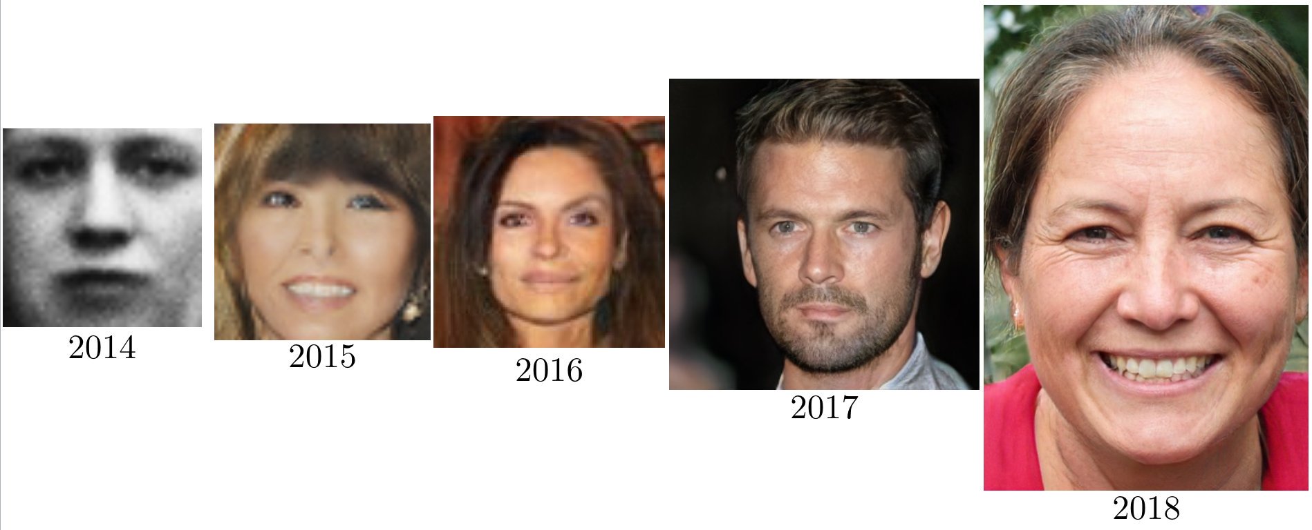
2014 (GAN) → 2015 (DCGAN) → 2016 (CoGAN) → 2017 (ProGAN) → 2018 (StyleGAN)
- Better error function
- LSGAN https://arxiv.org/abs/1611.04076
- RaGAN https://arxiv.org/abs/1807.00734
- GAN v2 (Feature Matching) https://arxiv.org/abs/1606.03498
- CGAN: Only one particular class generation (instead of blurry multiclass).
- InfoGAN: Disentaged representation (Dec. 2016, OpenAI)
- CycleGAN: Domain adaptation (Oct. 2017, Berkeley)
- SAGAN: Self-Attention GAN (May. 2018, Google)
- Relativistic GAN: Rethinking adversary (Jul. 2018, LD Isntitute)
- Progressive GAN: One step at a time (Oct 2017, NVIDIA)
- DCGAN: Deep Convolutional GAN (Nov. 2016, Facebook)
- BigGAN: SotA for image synthesis. Same GAN techiques, but larger. Increase model capacity & batch size.
- BEGAN: Balancing Generator (May. 2017, Google)
- WGAN: Wasserstein GAN. Learning distribution (Dec. 2017, Facebook)
- VAEGAN: Improving VAE by GANs (Feb. 2016, TU Denmark)
- SeqGAN: Sequence learning with GANs (May 2017, Shangai Univ.)
- Background-foreground segmentation so images simply slide behind objects in the front zone.
- Optical flow analysis helps determine the overall movement of virtual ads.
- Planar tracking helps smooth positioning.
- Image color adjustment is optimized according to the environment.
- Segmentation: Usually Loss = IoU + Dice + 0.8*BCE
- Pixel-wise cross entropy: each pixel individually, comparing the class predictions (depth-wise pixel vector)
- IoU (F0):
(Pred ∩ GT)/(Pred ∪ GT)=TP / TP + FP * FN - Dice (F1):
2 * (Pred ∩ GT)/(Pred + GT)=2·TP / 2·TP + FP * FN- Range from
0(worst) to1(best) - In order to formulate a loss function which can be minimized, we'll simply use
1 − Dice
- Range from
- Generation
- Pixel MSE: Flat the 2D images and compare them with regular MSE.
- Discriminator/Critic The loss function is a binary classification pretrained resnet (real/fake).
- Feature losses or perpetual losses.
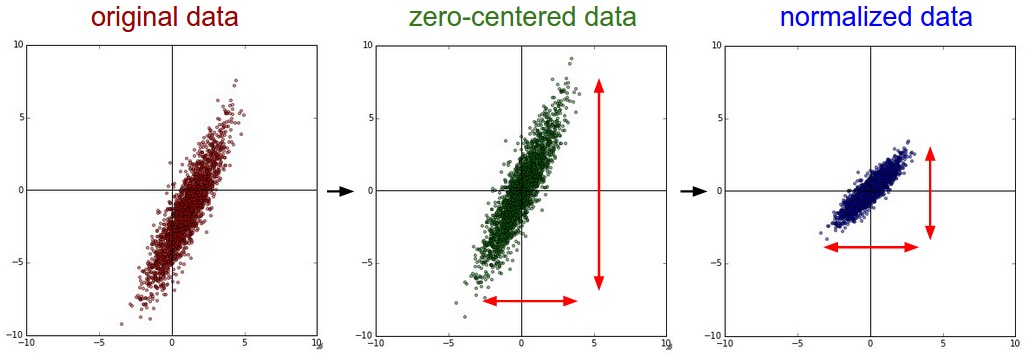
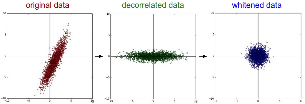
- Mean subtraction: Center the data to zero.
x = x - x.mean()fights vanishing and exploding gradients - Standardize: Put the data on the same scale.
x = x / x.std()improves convergence speed and accuracy
- Mean subtraction: Center the data in zero.
x = x - x.mean() - Decorrelation or PCA: Rotate the data until there is no correlation anymore.
- Whitening: Put the data on the same scale.
whitened = decorrelated / np.sqrt(eigVals + 1e-5)
- A year in computer vision
- Others
- Inceptionism
- Capsule net
- pyimagesearch: Start here
- GANs
- Pretrained models in pytorch
- Ranking,
- comparison paper
- Little tricks paper
- GPipe
