A module for analysing inter-event times (IETs) for time series observed inside a time window. The beginning and ending of the time window censors IETs of ongoing processes, and this censoring is done with higher probability for long IETs. This means that the observed IETs in a data can be much shorter than the real ones.
The motivation for creating this module comes from analysing temporal networks, but it can be used for any other event-based data consisting of a series of times stamps. In temporal networks, these would be, for example, time stamps at which edges or nodes are active.
This module was originally created for as part of a research project at the Mathematical Institute at the University of Oxford, which lead to the following publication where the methods used in this module are used:
- "Estimating interevent time distributions from finite observation periods in communication networks" M Kivelä, MA Porter. Physical Review E 92 (5), 052813
- The module is written for Python 2.7
- Depends on SciPy
The most important class in the module for analysing inter-event times is the IntereventTimeEstimator. For example, to create an estimator for temporal data with time window from 0 to 1, and where the data is assumed to come from a stationary process, you can use the commands: (see the documentation of the IntereventTimesEstimator for details on the arguments)
>>> import events
>>> estimator=events.IntereventTimeEstimator(1,mode="censorall")
The module can also be used to create event sequences using renewal processes. For example, to create an event sequence with a power-law inter-event time distribution with exponent 2.1 and smallest values 0.001, and creating estimates for the IET distributions you do the following:
>>> timeseq=events.generate_renewal_process_plaw(2.1,10**-3,1.0)
>>> estimator.add_time_seq(timeseq)
>>> estimator.get_naive_estimator() # Naive estimate of the cumulative distribution, only observed IETs are considered
>>> estimator.get_estimator() # Kaplan-Meier estimator for the cumulative IET distribution
The estimator object can pool together multiple event sequences, assuming that they all come from the same process. In the following we create in 999 additional time sequences and use all of them to estimate the IET distribution.
>>> from matplotlib import pyplot as plt
>>> for i in range(999): estimator.add_time_seq(events.generate_renewal_process_plaw(2.1,10**-3,1.0))
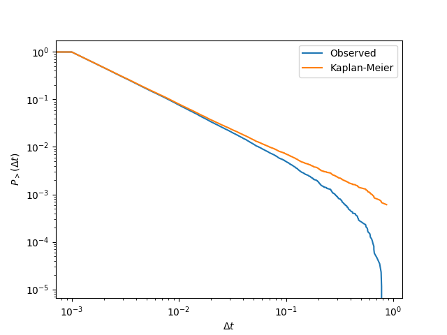
>>> plt.loglog(*estimator.get_naive_estimator(),label="Observed")
>>> plt.loglog(*estimator.get_estimator(),label="Kaplan-Meier")
>>> plt.legend()
>>> plt.xlabel(r"$\Delta t$")
>>> plt.ylabel(r"$P_>(\Delta t)$")
>>> plt.show()
A power-law distribution should show up as a straight line in log-log plot. This is indeed the case for the distribution estimated using the Kaplan-Meier estimator, but the IETs that are close to the the window width are cut out by the beginning and ending of the time window as seen in the Observed distribution.
- Mikko Kivela (bolozna@gmail.com)
