A Python package for approximate Bayesian inference with computationally-expensive models
approxposterior is a Python package for efficient approximate Bayesian
inference and Bayesian optimization of computationally-expensive models. approxposterior
trains a Gaussian process (GP) surrogate for the computationally-expensive model
and employs an active learning approach to iteratively improve the GPs predictive
performance while minimizing the number of calls to the expensive model required
to generate the GP's training set.
approxposterior implements both the Bayesian Active Learning for Posterior Estimation (BAPE, Kandasamy et al. (2017)) and Adaptive Gaussian process approximation for Bayesian inference with expensive likelihood functions (AGP, Wang & Li (2018)) algorithms for estimating posterior probability distributions for use with inference problems with computationally-expensive models. In such situations,
the goal is to infer posterior probability distributions for model parameters, given some data, with the additional constraint of minimizing the number of forward model evaluations given the model's assumed large computational cost. approxposterior trains a Gaussian Process (GP) surrogate model for the likelihood evaluation by modeling the covariances in logprobability (logprior + loglikelihood) space. approxposterior then uses this GP within an MCMC sampler for each likelihood evaluation to perform the inference. approxposterior iteratively improves the GP's predictive performance by leveraging the inherent uncertainty in the GP's predictions to identify high-likelihood regions in parameter space where the GP is uncertain. approxposterior then evaluates the forward model at these points to expand the training set in relevant regions of parameter space, re-training the GP to maximize its predictive ability while minimizing the size of the training set. Check out the BAPE paper by Kandasamy et al. (2017) and the AGP paper by Wang & Li (2018) for in-depth descriptions of the respective algorithms.
Check out the documentation at https://dflemin3.github.io/approxposterior/ for a more in-depth explanation about the code, detailed API notes, numerous examples with figures.
Using conda:
conda install -c conda-forge approxposteriorUsing pip:
pip install approxposteriorThis step can fail if george (the Python Gaussian Process package) is not properly installed and compiled. To install george, run
conda install -c conda-forge georgeFrom source:
git clone https://github.com/dflemin3/approxposterior.git
cd approxposterior
python setup.py installBelow is a simple application of approxposterior based on the Wang & Li (2017) example.
from approxposterior import approx, gpUtils, likelihood as lh, utility as ut
import numpy as np

# Define algorithm parameters
m0 = 50                           # Initial size of training set
m = 20                            # Number of new points to find each iteration
nmax = 2                          # Maximum number of iterations
bounds = [(-5,5), (-5,5)]         # Prior bounds
algorithm = "bape"                # Use the Kandasamy et al. (2017) formalism
seed = 57                         # RNG seed
np.random.seed(seed)

# emcee MCMC parameters
samplerKwargs = {"nwalkers" : 20}        # emcee.EnsembleSampler parameters
mcmcKwargs = {"iterations" : int(2.0e4)} # emcee.EnsembleSampler.run_mcmc parameters

# Sample design points from prior
theta = lh.rosenbrockSample(m0)

# Evaluate forward model log likelihood + lnprior for each theta
y = np.zeros(len(theta))
for ii in range(len(theta)):
    y[ii] = lh.rosenbrockLnlike(theta[ii]) + lh.rosenbrockLnprior(theta[ii])

# Default GP with an ExpSquaredKernel
gp = gpUtils.defaultGP(theta, y, white_noise=-12)

# Initialize object using the Wang & Li (2018) Rosenbrock function example
ap = approx.ApproxPosterior(theta=theta,
                            y=y,
                            gp=gp,
                            lnprior=lh.rosenbrockLnprior,
                            lnlike=lh.rosenbrockLnlike,
                            priorSample=lh.rosenbrockSample,
                            bounds=bounds,
                            algorithm=algorithm)

# Run!
ap.run(m=m, nmax=nmax, estBurnin=True, nGPRestarts=3, mcmcKwargs=mcmcKwargs,
       cache=False, samplerKwargs=samplerKwargs, verbose=True, thinChains=False,
       onlyLastMCMC=True)

# Check out the final posterior distribution!
import corner

# Load in chain from last iteration
samples = ap.sampler.get_chain(discard=ap.iburns[-1], flat=True, thin=ap.ithins[-1])

# Corner plot!
fig = corner.corner(samples, quantiles=[0.16, 0.5, 0.84], show_titles=True,
                    scale_hist=True, plot_contours=True)

# Plot where forward model was evaluated - uncomment to plot!
fig.axes[2].scatter(ap.theta[m0:,0], ap.theta[m0:,1], s=10, color="red", zorder=20)

# Save figure
fig.savefig("finalPosterior.png", bbox_inches="tight")
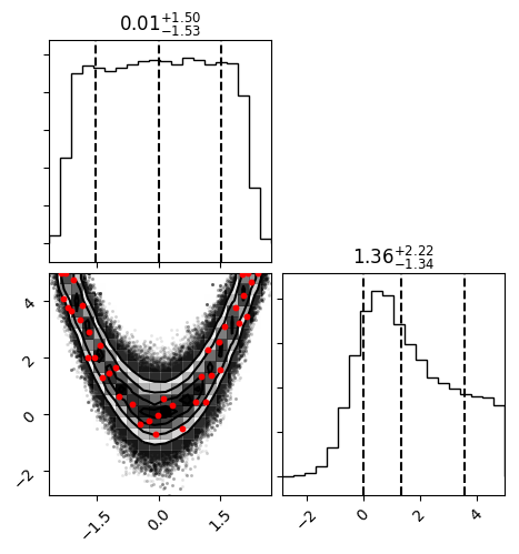
The final distribution will look something like this:
The red points were selected by approxposterior by maximizing the BAPE utility function.
At each red point, approxposterior ran the forward model to evaluate the true likelihood
and added this input-likelihood pair to the GP's training set. We retrain the GP each time
to improve its predictive ability. Note how the points are selected in regions of
high posterior density, precisely where we would want to maximize the GP's predictive ability! By using the
BAPE point selection scheme, approxposterior does not waste computational resources by
evaluating the forward model in low likelihood regions.
Check out the examples directory for Jupyter Notebook examples and explanations. Check out the full documentation for a more in-depth explanation of classes, methods, variables, and how to use the code.
If you would like to contribute to this code, please feel free to fork the repository, make some edits, and open a pull request. If you find a bug, have a suggestion, etc, please open up an issue!
If you use this code, please cite the following:
Fleming and VanderPlas (2018):
@ARTICLE{Fleming2018,
   author = {{Fleming}, D.~P. and {VanderPlas}, J.},
    title = "{approxposterior: Approximate Posterior Distributions in Python}",
  journal = {The Journal of Open Source Software},
     year = 2018,
    month = sep,
   volume = 3,
    pages = {781},
      doi = {10.21105/joss.00781},
   adsurl = {http://adsabs.harvard.edu/abs/2018JOSS....3..781P},
  adsnote = {Provided by the SAO/NASA Astrophysics Data System}
}
Kandasamy et al. (2017):
@article{Kandasamy2017,
title = "Query efficient posterior estimation in scientific experiments via Bayesian active learning",
journal = "Artificial Intelligence",
volume = "243",
pages = "45 - 56",
year = "2017",
issn = "0004-3702",
doi = "https://doi.org/10.1016/j.artint.2016.11.002",
url = "http://www.sciencedirect.com/science/article/pii/S0004370216301394",
author = "Kirthevasan Kandasamy and Jeff Schneider and Barnabás Póczos",
keywords = "Posterior estimation, Active learning, Gaussian processes"}
Wang & Li (2018):
@article{Wang2018,
author = {Wang, Hongqiao and Li, Jinglai},
title = {Adaptive Gaussian Process Approximation for Bayesian Inference with Expensive Likelihood Functions},
journal = {Neural Computation},
volume = {30},
number = {11},
pages = {3072-3094},
year = {2018},
doi = {10.1162/neco\_a\_01127},
URL = { https://doi.org/10.1162/neco_a_01127},
eprint = {https://doi.org/10.1162/neco_a_01127}}


