\maketitle
All enclosed documentation and data is available from Github at: https://github.com/jboes/amp-tutorial.git
- Similarly, the PDF can be found here: https://github.com/jboes/amp-tutorial/blob/master/workbook.pdf
- All of the code described within is open source with the exception of the Vienna ab initio simulation package (VASP).
- Have questions or are interested in learning more? Feel free to contact me at: jboes@andrew.cmu.edu.
In the Kitchin group, we use the VASP suit to perform Density functional theory (DFT) calculations.
- Solves the Kohn-Sham Equations which approximate the Schrodinger equation with electron density.
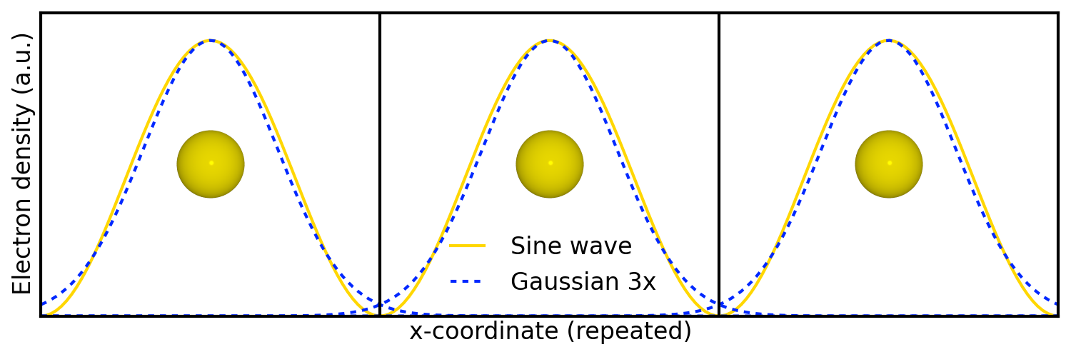
- VASP is ideal for bulk system since it uses plane waves to estimate the electron density.
- Although powerful and accurate DFT is too slow for more advanced application, such as molecular dynamics (MD) and larger unit cells.
- MD requires a large number of calculations in series, which DFT is poorly suited for.
Neural networks are a machine learning technique which can be use to construct a flexible function from an arbitrary input variable.
- This has been successfully implemented to predict potential energies (function output) from atomic positions (input variable).
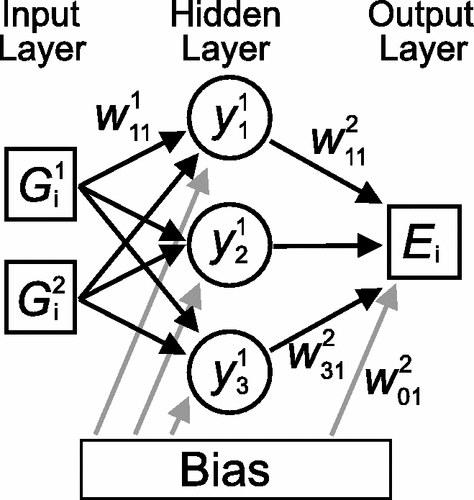
- A basic feed-forward neural networks is demonstrated in Figure ref:fig-nn for a 2 atom system.
- Feed-forward neural networks are limited by their construction. Atoms cannot be added or disordered using this method.
To use NNs on variable systems of atoms we need a different set of inputs than atomic positions.
- There are many ways to describe various atomic configurations other than Cartesian coordinates.
- Whatever descriptor we use needs to be accessible without performing a DFT calculation.
- Behler and Parrinello suggested a cutoff radius and “symmetry functions”.
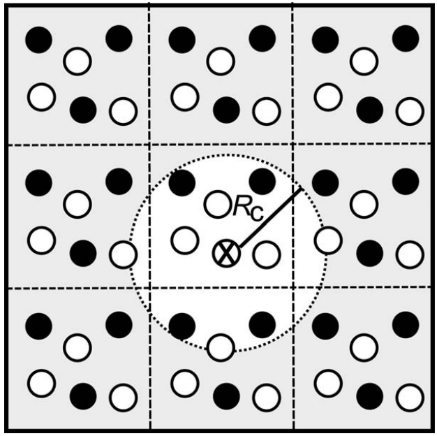
The cutoff radius $Rc$ is useful because it limits the size of the symmetry function required. This is demonstrated in Figure ref:fig-cutoff.
- Choice of $Rc$ is critical! We assume no interactions occur beyond this cutoff.
- This is not suitable for systems with long-range interactions.
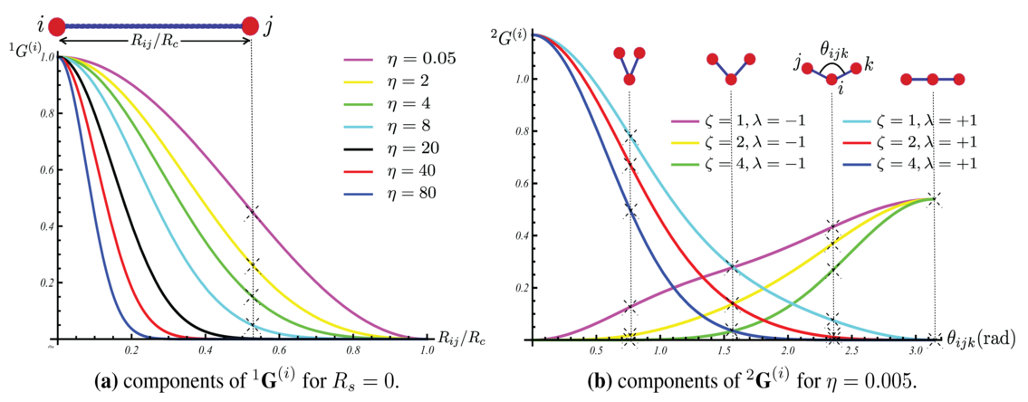
For each atom, we construct a “symmetry function” made of various Behler-Parrinello descriptors. Some of these descriptors are demonstrated in Figure ref:fig-behler.
- We can use as many descriptors as needed to define the system.
- Fewer is better since less variables makes the function smaller, which in turn computes faster.
Finally, for each atom in a system, we calculate the “symmetry function” and pass it to a general feed-forward NN as shown in Figure ref:fig-bpnn.
- Then we sum the energy contributions from each atom to get the total energy.
- More information can be found in Reference cite:behler-2007-gener-neural.
First, we need to determine an appropriate level of convergence for our calculations. I usually use the natural bulk configuration of a metal for these studies. For Pd, this is face centered cubic (fcc).
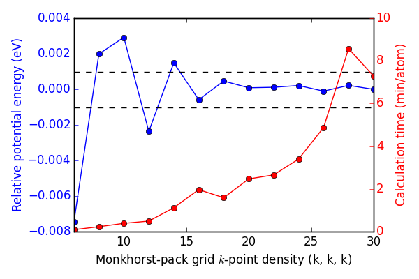
First, we determine an appropriate k-point convergence. We will be performing many calculations, so a high level of accuracy is desirable, but not if the computational cost is too high. I use a high energy cutoff (400 eV) to make sure there are no effects from encut convergence to potentially skew the results.
Figure ref:fig-kpts shows that a Monkhorst-pack grid of roughly (16, 16, 16) k-points is sufficient to each 1 meV convergence.
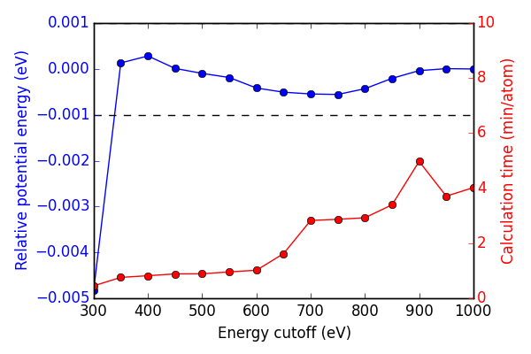
Next, we look at energy cutoff convergence. Similarly, k-point density is fixed at (16, 16, 16) for these calculations to ensure no effects from lack of convergence.
In this case, Figure ref:fig-encut shows 350 eV energy cutoff is sufficient to achieve 1 meV convergence.
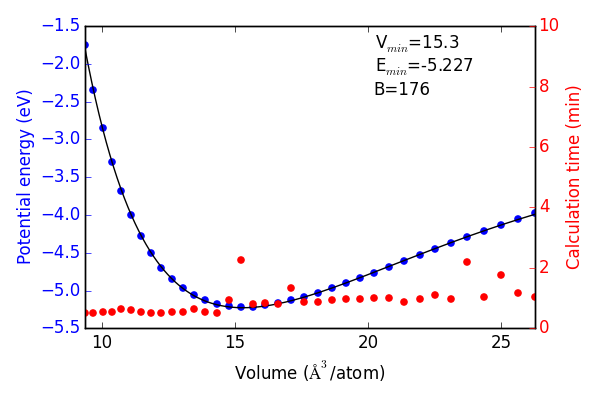
Next we use the convergence criteria to calculate Pd bulk fcc EOS at the desired level of accuracy. I have chosen (16, 16, 16) k-points, 350 eV encut. We will need a good sized sample to fit the neural network. I have chosen a fine grid of 71 points about the expected minimum in energy, and 29 additional points to span the space leading to “infinite” separation. Figure ref:fig-eos shows the resulting fit. The code block also generates an ASE database, which we will use from this point on for easy access to the data. It can be found in the Github repository mentioned in the introduction.
To train a neural network we will be using AMP (https://bitbucket.org/andrewpeterson/amp), a software package developed by the Peterson group at Brown University.
Before we begin creating out neural network, we need to separate about 10% of out data into a validation set. This will be useful later, when determining whether over fitting has occurred. There is functionality for this in AMP, but it does not provide with as much control as the following code.
Now we have sudo-randomly labeled 10% of our calculations for validation, and the rest are waiting to be trained in the new train.db file.
For all of out neural networks, we will be using the Behler-Parenello (BP) framework for distinguishing between geometries of atoms. Little to no work is published on how to systematically chose an appropriate number of variables for your BP framework, so we simply use the default settings in AMP for now. However, it is worth mentioning that a single G1 type variable (simplest possible descriptor) could be used to describe the fcc EOS, if that is all we are interested in.
We also need to define a cutoff radius for our system which will determine the maximum distance that the BP framework considers atoms to be interacting. 6
Finally, it is also often desirable to have multiple neural networks which are trained to the same level of accuracy, but with different frameworks. These frameworks are determined by the number of nodes and hidden layers used. In general, we want the smallest number of nodes and layers possible to avoid the possibility of over fitting. However, too small a framework will be too rigid to properly fit complex potential energy surfaces.
These jobs can be run locally:
For the sake of reproducibility. I have separately generated a starting point above for both framework. Now, I use the initial guess previously found to initiate the fitting process:
Once the calculations finish we can check their convergence using the code below. These are trivial networks to train, so convergence should not be an issue. This can be a difficult and time consuming part of the process for more complex system.
| Hidden layers | Iteration | Time | Cost Function | Energy RMSE |
|---|---|---|---|---|
| {u’Pd’: [2, 2]} | 134 | 2016-06-27T16:00:34 | 4.854e-05 | 9.953e-04 |
| {u’Pd’: [2, 3]} | 277 | 2016-06-27T16:00:47 | 4.821e-05 | 9.919e-04 |
The single atom unit cell enforces perfect symmetry. This results in cancellation of forces on the atom in the unit cell. Hence, force RMSE = 0.0, which makes for fast training, but less information to train too.
Now we need to validate our results to ensure that no over fitting has occurred. First, we will look at the residuals to the training and validation data. Then we will see if the neural networks perform well for their intended purpose. For ease of access, we will add the neural network energy predictions to the database for each structure.
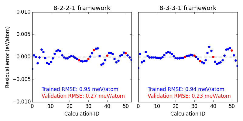
First we look at the residual errors of all the data in the database for each of our frameworks shown in Figure ref:fig-residuals-1. For both fits, the validation set has lower RMSE than the training set. This is a good indication that neither has been over fit, which we can also observe for this simple example, since the validation points follow the same trends observed for the training set data. This is also a good example of how adding additional, unnecessary elements to the framework leads to lower overall fitting accuracy.
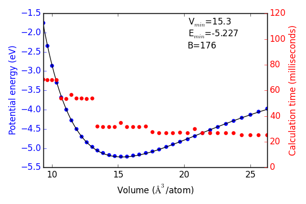
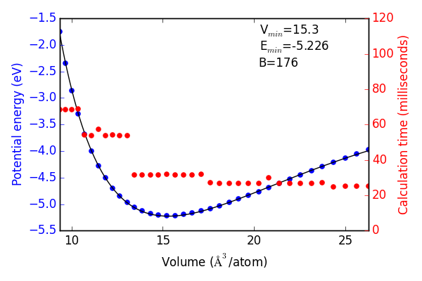
Next, we recreate the equation of state using both of the neural networks and the same methodology as with DFT. The results are shown in Figures ref:fig-eos-NN2 and ref:fig-eos-NN3 for the 2-2 and 3-3 frameworks, respectively.
Each neural network creates an excellent fit to the DFT data, and we see that the calculation speed has improved by up to 6 orders of magnitude in the most extreme cases. For this application the choice of framework seems to have little effect on the equation of state produced.
Now we can try and apply our neural networks to things it was not fit to.
For this, we will use or two neural networks jointly which will save us a good amount of time validating the networks as we begin to extrapolate. This is demonstrated in the next section.
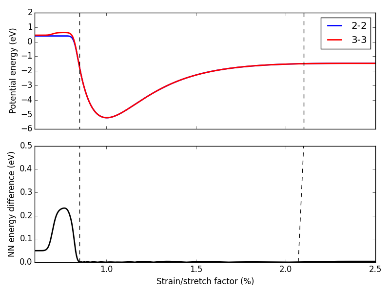
First, we expand the region of equation of state to see how well it extrapolates. In Figure ref:fig-app-eos, we expand the region of the original equation of state beyond the black dashed lines.
At extreme stretch (factor > 2.1%) both neural networks agree because we have trained it nearly to the cutoff radius of 6.0
As soon as we strain the lattice below the trained region, the network predictions quickly diverge. This indicates that the training set is not useful for predictions in this region.
We performed 1,000 calculations to produce this figure. To have validated all 1,000 points with DFT would be too time consuming. Instead, we rely on disagreement between neural networks with different framework to probe poorly fitted regions.
Here we attempt to calculate the vacancy formation energy for fcc Pd. This is calculated as shown in Equation ref:eqn-vac.
\begin{eqnarray} E_v = E_f - \frac{n_i - 1}{n_i} E_i \label{eqn-vac} \end{eqnarray}
from the literature cite:mattsson-2002-calcul, we know that DFT-GGA should predict a vacancy formation energy of about 1.50 eV.
- Vacancy formation energy with 2-2 framework NN: 4.170 eV
- Vacancy formation energy with 3-3 framework NN: 0.411 eV
neither network does a good job predicting the vacancy formation energy. This is because the networks do not know how to calculate the energy of an fcc lattice with a missing atom.
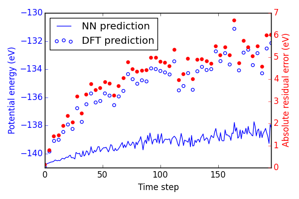
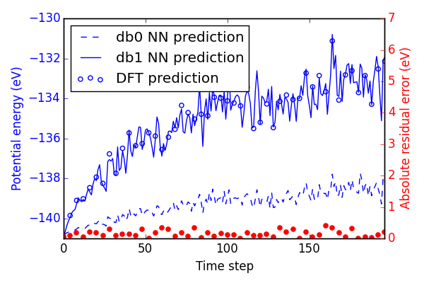
Finally, we try an MD simulation. In Figure ref:fig-MD1 we begin with a 3 × 3 × 3 primitive unit cell of Pd and add a random amount of kinetic energy to each of the 27 atoms in the system. We then use the forces on those atoms to determine where they will be after a small forward step in time (5 fs). Then, we use the BPNN to calculate the energy and forces on the perturbed system and repeat for 200 time steps.
In Figure ref:fig-MD1, the NN energy and corresponding DFT energy of every 4th step is shown. Although the NN predicts the upward trend in energy correctly, the residuals are quite large. This is likely not an acceptable level of error for most applications.
Here we perform a second iteration of the neural network. Now we will include the DFT validation calculations on the MD simulation shown in Figure ref:fig-MD1. The first two sections are repetitions of previous training code shown above.
Training the second networks took significantly longer since we are no longer training such simple structures. There is now a need for more than one descriptor to define the system. However, 8 descriptors is the default for a single element.
We submit these to the queue on Gilgamesh, since they are much longer to run:
| Hidden layers | Iteration | Time | Cost Function | Energy RMSE | Force RMSE |
|---|---|---|---|---|---|
| {u’Pd’: [2, 2]} | 5716 | 2016-06-30T17:48:06 | 3.866e-02 | 4.999e-03 | 1.965e-01 |
| {u’Pd’: [2, 3]} | 4539 | 2016-07-01T12:33:17 | 3.661e-02 | 4.715e-03 | 1.916e-01 |
Since volume is no longer a good description of all structures in our data set, we will simply perform validation of residuals errors based on calculation IDs.
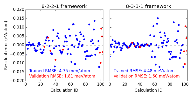
Figure ref:fig-residuals-2 shows that the second iteration of the fit is not as accurate as the first. This is because we have expanded the scope of the potential energy surface we are trying to fit to. Additional accuracy can be obtained by further sampling of similar structures, in this region of the potential energy surface. For most current applications with NN, an RMSE of
If we re-calculate the energy of the MD trajectory from Figure ref:fig-MD1, we can see in Figure ref:fig-MD2 that the predictions are greatly improved. Note that the scale of absolute residuals on the right is an order of magnitude lower than before.
Normalizing these residuals on a per atom basis gives absolute residuals errors below 5 meV/atom. This is considered an acceptable level of error for most applications in the literature, but will not be sufficient for all purposes still. Training large systems of atoms to even higher levels of accuracy will become quite difficult since AMP works on a cost function normalized by the number of atoms in each system. This preferentially results in lower levels of absolute residual error for small systems.
bibliographystyle:unsrt bibliography:./bibliography.bib
