A modern Fortran library providing an object-oriented approach to solving and exploring ordinary differential equations.
The documentation can be found here.
- Runge-Kutta, 5th Order (Dormand-Prince)
- Runge-Kutta, 3rd Order (Bogacki-Shampine)
- Runge-Kutta, 8th Order (Hairer, Nörsett, & Wanner)
- Rosenbrock, 4th Order
CMakeThis library can be built using CMake. For instructions see Running CMake.
FPM can also be used to build this library using the provided fpm.toml.
fpm buildThe DIFFEQ library can be used within your FPM project by adding the following to your fpm.toml file.
[dependencies]
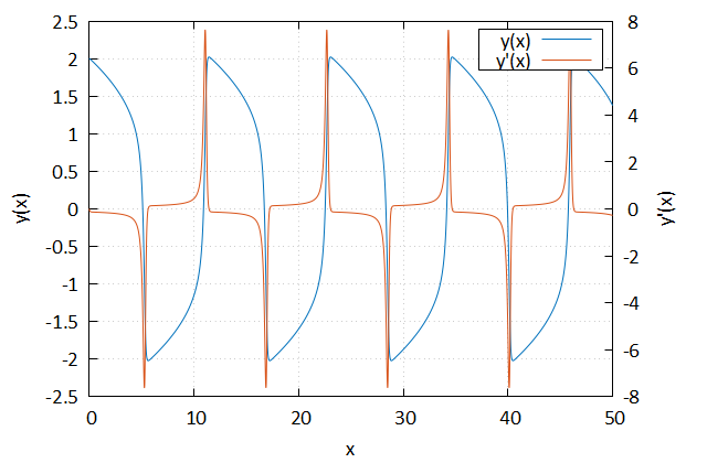
diffeq = { git = "https://github.com/jchristopherson/diffeq" }The following example illustrates solving the Van der Pol equation using a 4th-order Rosenbrock solver, but other solvers can be used in an identical manner. The example also utilizes the FPLOT library to plot the solution.
program example
    use iso_fortran_env
    use diffeq
    use diffeq_models
    use fplot_core
    implicit none

    ! Local Variables
    type(rosenbrock) :: integrator
    type(ode_container) :: mdl
    real(real64), allocatable :: sol(:,:)

    ! Plot Variables
    type(plot_2d) :: plt
    type(plot_data_2d) :: pd1, pd2
    class(plot_axis), pointer :: xAxis, yAxis, y2Axis
    class(legend), pointer :: lgnd

    ! Define the model
    mdl%fcn => vanderpol

    ! Compute the solution
    call integrator%solve(mdl, [0.0d0, 5.0d1], [2.0d0, 0.0d0])
    sol = integrator%get_solution()

    ! Plot the results
    call plt%initialize()
    xAxis => plt%get_x_axis()
    yAxis => plt%get_y_axis()
    y2Axis => plt%get_y2_axis()
    lgnd => plt%get_legend()
    call xAxis%set_title("x")
    call yAxis%set_title("y(x)")
    call y2Axis%set_title("y'(x)")
    call plt%set_use_y2_axis(.true.)
    call lgnd%set_is_visible(.true.)

    call pd1%define_data(sol(:,1), sol(:,2))
    call pd1%set_name("y(x)")
    call plt%push(pd1)

    call pd2%define_data(sol(:,1), sol(:,3))
    call pd2%set_draw_against_y2(.true.)
    call pd2%set_name("y'(x)")
    call plt%push(pd2)

    call plt%draw()
end program
The routine containing the ODE is located in a different module for this example. This routine is as follows.
pure subroutine vanderpol(x, y, dydx)
    ! Arguments
    real(real64), intent(in) :: x, y(:)
    real(real64), intent(out) :: dydx(:)

    ! Model Constants
    real(real64), parameter :: mu = 5.0d0

    ! Equations
    dydx(1) = y(2)
    dydx(2) = mu * (1.0d0 - y(1)**2) * y(2) - y(1)
end subroutine
Here's another example comparing the behavior of several integrators for the same Van der Pol problem illustrated in the previous example. In this example it can be seen that all of the integrators can be utilized in an identical manner. Additionally, this example illustrates the use of a PI-type controller for step-size control. Such a controller can be beneficial in the event stability issues are encountered during solution; however, this benefit usually comes with a drawback of decreased efficiency. For this reason, the default behavior for any of the solvers is to not utilize any PI control; however, it is available if needed.
program example
    use iso_fortran_env
    use diffeq
    use diffeq_models
    implicit none

    ! Initial Conditions & Time Constraints
    real(real64), parameter :: t(2) = [0.0d0, 5.0d1]
    real(real64), parameter :: ic(2) = [2.0d0, 0.0d0]

    ! Local Variables
    type(runge_kutta_23) :: integrator_1
    type(runge_kutta_45) :: integrator_2
    type(runge_kutta_853) :: integrator_3
    type(rosenbrock) :: integrator_4
    type(ode_container) :: mdl
    real(real64), allocatable, dimension(:,:) :: s1, s2, s3, s4, s5

    ! Define the model
    mdl%fcn => vanderpol

    ! Integrate the model with each integrator
    call integrator_1%solve(mdl, t, ic)
    call integrator_2%solve(mdl, t, ic)
    call integrator_3%solve(mdl, t, ic)
    call integrator_4%solve(mdl, t, ic)

    ! Retrieve the solution from each integrator
    s1 = integrator_1%get_solution()
    s2 = integrator_2%get_solution()
    s3 = integrator_3%get_solution()
    s4 = integrator_4%get_solution()

    ! Print out the size of each solution
    print "(AI0A)", "RUNGE_KUTTA_23: ", size(s1, 1), " Solution Points"
    print "(AI0A)", "RUNGE_KUTTA_45: ", size(s2, 1), " Solution Points"
    print "(AI0A)", "RUNGE_KUTTA_853: ", size(s3, 1), " Solution Points"
    print "(AI0A)", "ROSENBROCK: ", size(s4, 1), " Solution Points"

    ! Now, implement a PI controller and check its effect.  This will likely
    ! increase the number of steps (loss of efficiency), but if there were
    ! any stability issues, stability will likely improve.  Stability is likely
    ! not relevant on this problem, but it's here for illustration purposes.
    call integrator_4%set_step_size_control_parameter(0.1d0)
    call integrator_4%solve(mdl, t, ic)
    s5 = integrator_4%get_solution()
    print "(AI0A)", "ROSENBROCK w/ PI Controller: ", size(s5, 1), " Solution Points"
end program
RUNGE_KUTTA_23: 2465 Solution Points
RUNGE_KUTTA_45: 583 Solution Points
RUNGE_KUTTA_853: 925 Solution Points
ROSENBROCK: 1178 Solution Points
ROSENBROCK w/ PI Controller: 2356 Solution PointsHere is a list of external code libraries utilized by this library. The CMake build script will include these dependencies automatically; however, it is highly recommended that an optimized BLAS and LAPACK already reside on your system for best performance (used by LINALG for linear algebra calculations).
- Butcher, J. C. (2003). Numerical methods for ordinary differential equations. J. Wiley.
- Shampine, L. F., & Reichelt, M. W., (1997). The MATLAB ODE suite. SIAM Journal on Scientific Computing. 18. 10.1137/S1064827594276424.
- J.R. Dormand, P.J. Prince (1980). A family of embedded Runge-Kutta formulae, Journal of Computational and Applied Mathematics, Volume 6, Issue 1, Pages 19-26, ISSN 0377-0427, https://doi.org/10.1016/0771-050X(80)90013-3.
- P. Bogacki, L.F. Shampine (1989). A 3(2) pair of Runge - Kutta formulas, Applied Mathematics Letters, Volume 2, Issue 4, Pages 321-325, ISSN 0893-9659, https://doi.org/10.1016/0893-9659(89)90079-7.
- Dormand, J. R. (1996). Numerical methods for differential equations a computational approach. CRC Press.
- Kennedy, C. A., Carpenter, M. H. (2016, March). Diagonally Implicit Runge-Kutta Methods for Ordinary Differential Equations. A Review. https://ntrs.nasa.gov/api/citations/20160005923/downloads/20160005923.pdf
- Stal, J. (2015). Implementation of Singly Diagonally Implicit Runge-Kutta Methods with Constant Step Sizes. https://core.ac.uk/download/pdf/289938621.pdf
- Nayfeh, A. H., & Balachandran, B. (1995). Applied Nonlinear Dynamics: Analytical, Computational, and Experimental Methods. J. Wiley.
