Efficient covariance computations for Adaptive Optics in Python
In Adaptive Optics control/estimation/simulations, it's common to find yourself performing an operation similar to:
import numpy as np
import aotools

# define some grid coordinates in x and y
n = 64
xx, yy = np.meshgrid(np.arange(n), np.arange(n), indexing="xy")
xx = xx.flatten()
yy = yy.flatten()

# compute the distances between every pair of coordinates in this grid
rr = ((xx[:, None]-xx[None, :])**2 + (yy[:, None]-yy[None, :])**2)**0.5

# evaluate the covariance at all points in
r0 = 0.15
L0 = 25.0
cov = aotools.phase_covariance(rr, r0, L0)
The goal of this package is to address 2 main limitations of this simple operation:
- The evaluation of the covariance function is highly parallelisable, though the implementation above is limited to CPU execution.
- The distance matrix (
rrin this case) is highly redundant, with many repeated values due to the regular geometry of the inputs.
These problems are addressed simultaneously by:
- using PyTorch to execute von Karman covariance functions on (e.g.) GPU, by simply defining a device to execute on. Note that PyTorch must be installed with the appropriate configuration, though for modern CUDA GPU devices, this is done by default. Just use
device="gpu"when you callaocov.phase_covariance. - calculating the unique elements of the distance matrix, and only evaluating the covariance function for these values, then copying the values for all other duplicated values.
Modifying the above example, we would instead use:
import numpy as np
import aocov # <-- import this package

# define some grid coordinates in x and y
n = 64
xx, yy = np.meshgrid(np.arange(n), np.arange(n), indexing="xy")
xx = xx.flatten()
yy = yy.flatten()

# compute the distances between every pair of coordinates in this grid
rr = ((xx[:, None]-xx[None, :])**2 + (yy[:, None]-yy[None, :])**2)**0.5

# evaluate a von Karman covariance on GPU
r0 = 0.15
L0 = 25.0
cov = aocov.phase_covariance(rr, r0, L0, device="cuda:0")
Furthermore, since the distance computations can become expensive, and is prone to typos, we provide a further convenience function, phase_covariance_xyxy. Finally, the example becomes:
import numpy as np
import aocov # <-- import this package

# define some grid coordinates in x and y
n = 64
xx, yy = np.meshgrid(np.arange(n), np.arange(n), indexing="xy")
xx = xx.flatten()
yy = yy.flatten()

# evaluate a von Karman covariance on GPU
r0 = 0.15
L0 = 25.0
cov = aocov.phase_covariance_xyxy(xx, yy, xx, yy, r0, L0, device="cuda:0")
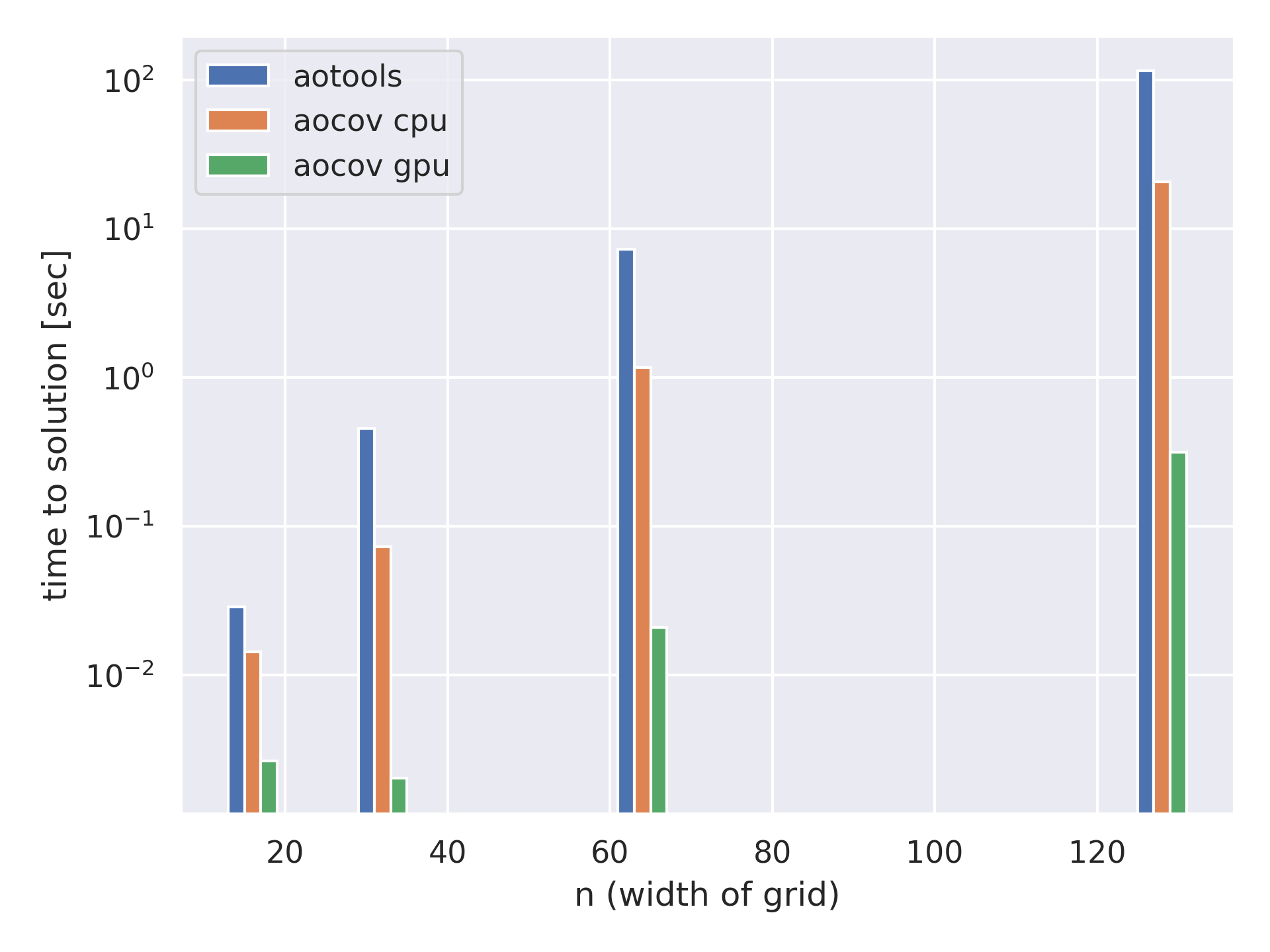
Note that the last option is likely to perform the fastest, see performance comparison below. Also, for the time being, PyTorch does not implement the required bessel function (scipy.special.kv(nu,x)), so the code makes a single call to the scipy function on CPU. If someone makes a torch-friendly version of kv(nu,x), this would further improve the performance of this module - especially on GPU.
For the latest version, simply clone and install this git repo using pip.
git clone git@github.com:jcranney/aocov
cd aocov
pip install -e .
If you are happy with a stable version, you can directly pip install:
pip install aocovThis repo comes with a performance test script perf/perf_test.py, you can tweak it to match your system dimensions. Note that
| n | elements |
|---|---|
| 16 | 65,536 |
| 32 | 1,048,576 |
| 64 | 16,777,216 |
| 128 | 268,435,456 |
Using the default parameters on a system 40 cores and a Tesla V100 32GB GPU, I measured the following:
| n | device | experiment | sec/matrix |
|---|---|---|---|
| 16 | cpu | no pytorch | 2.880e-02 |
| 16 | cpu | rr in numpy, rest in aocov | 1.222e-02 |
| 16 | cpu | all in aocov | 1.435e-02 |
| 16 | cuda:0 | rr in numpy, rest in aocov | 1.110e+00 |
| 16 | cuda:0 | all in aocov | 2.640e-03 |
| 32 | cpu | no pytorch | 4.535e-01 |
| 32 | cpu | rr in numpy, rest in aocov | 8.379e-02 |
| 32 | cpu | all in aocov | 7.282e-02 |
| 32 | cuda:0 | rr in numpy, rest in aocov | 8.874e-03 |
| 32 | cuda:0 | all in aocov | 2.020e-03 |
| 64 | cpu | no pytorch | 7.233e+00 |
| 64 | cpu | rr in numpy, rest in aocov | 1.269e+00 |
| 64 | cpu | all in aocov | 1.159e+00 |
| 64 | cuda:0 | rr in numpy, rest in aocov | 1.777e-01 |
| 64 | cuda:0 | all in aocov | 2.087e-02 |
| 128 | cpu | no pytorch | 1.143e+02 |
| 128 | cpu | rr in numpy, rest in aocov | 2.218e+01 |
| 128 | cpu | all in aocov | 2.056e+01 |
| 128 | cuda:0 | rr in numpy, rest in aocov | 2.560e+00 |
| 128 | cuda:0 | all in aocov | 3.152e-01 |
For
