About the project

An Kalman-Bucy filter implementation in JAX started from a fork of jaxman with extensions. One extension considers non equidistant "time" steps, ie. non constante transport F matrix and perturbation Q matrix. In the notation of wikipedia.

Getting started

Follow the below instructions in order to get started.

Prerequisites

Start by installing JAX.

Installation

The library is currently not available on pypi, and there are currently no plans on releasing it there.

Usage

Beyond the original KalmanFilter (alias to KalmanFilterStd) class that deals with equaly spaced observations, the extension provides KalmanFilterNonEquid class, then one provides functions to get the transport matrix F and transport covariance matrix Q

from jaxkalm import KalmanFilterNonEquid
import jax.random as jaxrnd
import matplotlib.pyplot as plt
import jax.numpy as jnp
import jax.scipy as jsc
from jax.scipy import optimize

#simple linear modeling to generate a dataset
def mean_fn(t,p):
    return p[0] + p[1]*t

#this loss function is used by BFGS-optimize to compare with Kalman filetring
def lik(p,xi,yi, sigma_obs):
    resid = mean_fn(xi, p)-yi
    return 0.5*jnp.sum((resid/sigma_obs) ** 2) 

#Random gene
rng_key = jaxrnd.PRNGKey(10)
rng_key, rng_key0 = jaxrnd.split(rng_key)

#dataset (t,y)_i
tMes = jax.random.uniform(rng_key0,minval=0.,maxval=20.0,shape=(30,))
tMes=jnp.sort(tMes)
par_true = jnp.array([0.1,0.2])
sigma_obs = 0.3
yMes = mean_fn(tMes,par_true) + sigma_obs * jaxrnd.normal(rng_key0,shape=tMes.shape)

#BFGS minisation
bfgs_fit= optimize.minimize(lik, jnp.array([0.,0.]),
                               args=(tMes,yMes,sigma_obs), method='BFGS', tol=1e-6, options=None)
p_fit = bfgs_fit.x # parameter fitted
y_fit = mean_fn(tMes, p_fit) # (t,y(t)) from fitted model

#Kalman
# The vector state is  X=(y,dy/dx)^T
#

# prediction: transport matrix k-1 -> k of state vector  (F mtx)
# dt is the difference of "time" between the next obsservation and the current state
def trans_mat_func(dt: float) -> jnp.array:
   return  jnp.array([[1., dt],[0.,1.]]) 
def trans_cov_func(dt: float) -> jnp.array:    # (Q mtx)
    return jnp.zeros(shape=(2,2))   #no perturbation during prediction


# observation aka measurements
obs_mat = jnp.array([1.0,0.])              # H projection matrix from mesurement to vector state (the measure is y_mes only)
obs_cov = sigma_obs**2                     # error (here 1D) on mesurement (R matrix)

# prepare Kalman filter
kf = KalmanFilterNonEquid(trans_mat_func, trans_cov_func,
                              obs_mat, obs_cov) 


result = kf.filter(yMes,tMes)             # iterate the kalman filtering automatic init.

#for the plot see the file ./tests/test_predict_function.py

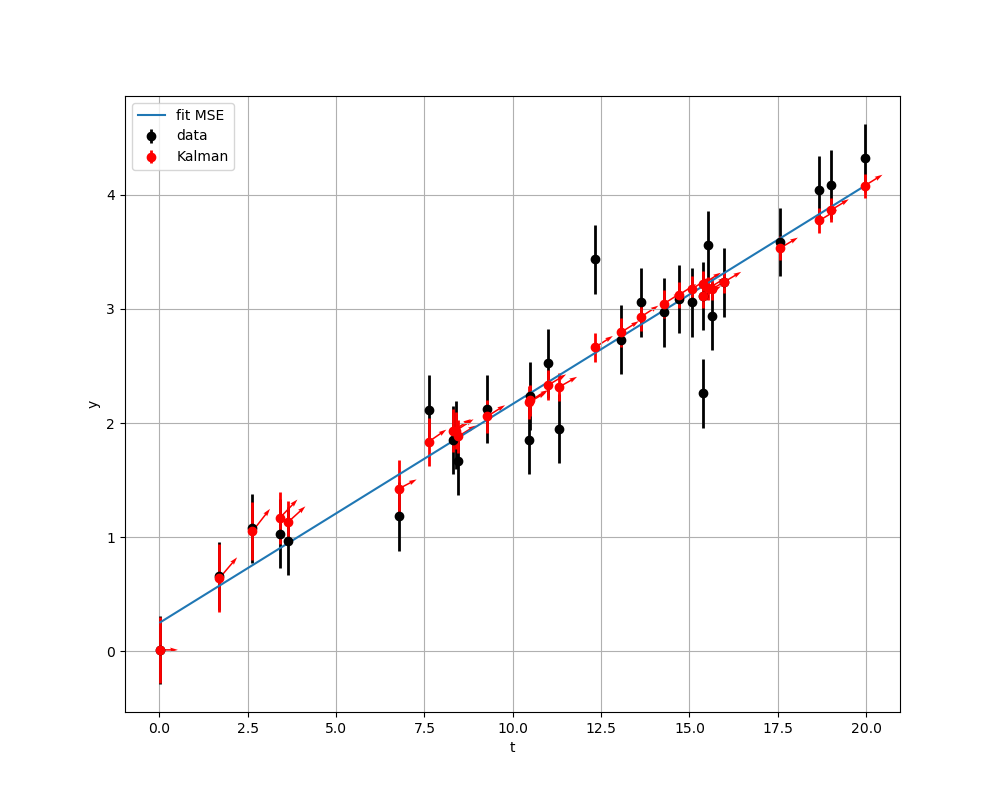
Resulting in the following pretty picture

Disclaimers