Advanced Lane Finding Project
The goals / steps of this project are the following:
- Compute the camera calibration matrix and distortion coefficients given a set of chessboard images.
- Apply a distortion correction to raw images.
- Use color transforms, gradients, etc., to create a thresholded binary image.
- Apply a perspective transform to rectify binary image ("birds-eye view").
- Detect lane pixels and fit to find the lane boundary.
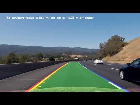
- Determine the curvature of the lane and vehicle position with respect to center.
- Warp the detected lane boundaries back onto the original image.
- Output visual display of the lane boundaries and numerical estimation of lane curvature and vehicle position.
The pipeline works steadily. The points used to approximate the lanes are shown as well as the curvature radius.
On the challenge-video, the nearby lanes are detected steadily. But, the distant lanes aren't detected, thus the polynomial lanes wobble a bit.

Rubric Points
1. Briefly state how you computed the camera matrix and distortion coefficients. Provide an example of a distortion corrected calibration image.
The code for this step is contained in the first and second code cell of the IPython notebook
I start by preparing "object points", which will be the (x, y, z) coordinates of the chessboard corners in the world. Here I am assuming the chessboard is fixed on the (x, y) plane at z=0, such that the object points are the same for each calibration image. Thus, objp is just a replicated array of coordinates, and objpoints will be appended with a copy of it every time I successfully detect all chessboard corners in a test image. imgpoints will be appended with the (x, y) pixel position of each of the corners in the image plane with each successful chessboard detection.

I then used the output objpoints and imgpoints to compute the camera calibration and distortion coefficients using the cv2.calibrateCamera() function. I applied this distortion correction to the test image using the cv2.undistort() function and obtained this result:

Comparing the two is rather difficult, but the hood of the car reveals the effect.
Further explanations may be obtained both from the openCV documentation and my udacity-forked camera calibration github repo
All camera images get undistorted as a first step. This enables me to calculate physical values out of any well-calibrated camera, even a fish-eyed gopro gets feasable.
2. Describe how (and identify where in your code) you used color transforms, gradients or other methods to create a thresholded binary image. Provide an example of a binary image result.
I used color thresholds to generate a binary image. The pipeline can be tuned using ipwidgets (Notebook part 5). I added two very difficult pictures of the video and added them to the example videos. This enabled me to tune the filters very fast and efficiently. After experimenting a lot with the S-channel of HSV pictures, the r-channel of the RGB-format, soebel-gradients and magnitude-gradients, I decided to look into other formats. The sobel-gradients are based on the unfiltered s-channel. I used the following parameters:
| Parameter | Value |
|---|---|
| sobel_kernel | 15 |
| sobel | 30:100 |
| saturation | 170:255 |
| red | 220:255 |
With this configuration, it is difficult to detect the shadowy parts of the lanes, because the S-Channel gets saturated. I tried to combine the parameters, that any 2 detected pixels would activate the resulting binary output.
After experimenting with different formats, the L channel from a “LUV” field detects the white lines and the B-channel from a LAB field detects yellow. This change enabled me to detect the near lanes of the challenge video. The thresholds for LUV are 210:255 and for LAB are 150:255.
 In the example, the red channel represents the gray-scale image in order to easily recognize the original image.
3. Describe how (and identify where in your code) you performed a perspective transform and provide an example of a transformed image.
The code for my perspective transform includes a function called birds_eye(), which appears in the 7th cell. The birds_eye() function takes as inputs an image (img), as well as source (src) and destination (dst) points. I chose the hardcode the source and destination points in the following manner:
left1=(100,700)
left2=(500,450) #further away
right1=(1180,700)
right2=(780,450) #further away

offset=400
dleft1=left1
dleft2=(left2[0]-offset,0)
dright1=right1
dright2=(right2[0]+offset,0)
This resulted in the following source and destination points:
| Source | Destination | Description |
|---|---|---|
| 100,700 | 100,700 | near left |
| 500,450 | 500, 50 | far left |
| 1180, 700 | 1180, 700 | near right |
| 780, 540 | 780,940 | far right |
I verified that my perspective transform was working as expected by drawing the src and dst points onto a test image and its warped counterpart to verify that the lines appear parallel in the warped image.


The 8th field of the notebook desribes the video pipeline class. It consists of birds_eye, find_lanes, update_lanes, append_and_pop_points, drawLine, mean_lanes, curve_radius and process_image. The function process_image serves as a main routine which will be called both on single frames or videos. The output is shown in the following picture:

First, the function undistorts the image. The birds_eye function gives the perspective from aboove.
 It is then binarized in the previosuly tuned pipeline
 binary_image as shown in the following image:

If either the left or the right lane is missing, the function find_lanes is called, else only update_lanes. Both functions are very similar to the examples provided in the class.
After the points are saved in their lists, append_and_pop_points caches them into class variables. The parameter filter_length defines how many results are stored in the cache. Longer storage gives a robust lane finding because more frames are analyzed.
The curve radius is also calculated based on the cached points. It is evaluated in the mean of all y-axis points, because a polynom tends to interpolate well, but it may be wrong in the outer part. For a polynom of a second order, the curve radius is a constant, then it doesn't matter where it is evaluated.
The inner polynom optically bends better, therefore the outer radius is discarded.
The function drawline adds the information in the returned frame. Showing the points used for the polynom explains the algorithm and helps to debug the filter and the algorithm. Therefore, it is added.
Testing the pipeline on every image serves as a verification. The class is initialized between every frame to avoid mixing lanes.

Describe how (and identify where in your code) you calculated the radius of curvature of the lane and the position of the vehicle with respect to center.
The pipeline class contains the function curve_radius. An experimentally gained factor from the udacity classrom transforms pixels into meters. Then, a polynom is fitted and the formula from this tutorial as shown in the picture is applied. Analyzing the results frame by frame, the outer lane tends to look very straight because of the camera transformation. The inner curve usually contains the better result. Therefore, the smaller value is stored in the cached list. The last 10 values are used to approximate the curvature.

The offset of the center is the difference between the middle of the lane and the vehicle position. The corresponding code is as follows.
        lane_midpoint = (np.polyval(left, 720)+np.polyval(right,720))*0.5
        vehicle_position  = image.shape[1]*0.5
dx=(vehicle_position-lane_midpoint)*xm_per_pix 1. Briefly discuss any problems / issues you faced in your implementation of this project. Where will your pipeline likely fail? What could you do to make it more robust?
The pipeline works well using the project video. The lines are steady. A filter length of 3 gives a fast reaction, whereas a filter length of 10 gives a very stable behaviour. It is therefore chosen.
In the challenge video, the nearby lanes are detected correctly. If the detected lanes are shortened, they serve as a robust input for a car control. Tthe extrapolated polynom doesn't fit well, because the points in the distance aren't detected by the algorithm. The harder challenge video shows the issues that need to be adressed. The main issues are:
- Reflexions
- Tight corners due to the hardcoded areas of the picture
- Changes in lightning due to the sun and the weather
- Rain, snow
- Slopes
- Bumpy roads and a moving car ...