The project teaches a DQN in a banana-collecting environment. The agent navigates in an environment to collect yellow bananas while avoiding black ones. A trained agent may act like this example:
A reward of +1 is provided for collecting a yellow banana, and a reward of -1 is provided for collecting a blue banana. Thus, the goal of your agent is to collect as many yellow bananas as possible while avoiding blue bananas.
The state space has 37 dimensions and contains the agent's velocity, along with ray-based perception of objects around agent's forward direction. Given this information, the agent has to learn how to best select actions. Four discrete actions are available, corresponding to:
0- move forward.1- move backward.2- turn left.3- turn right.
The task is episodic, and in order to solve the environment, the agent must get an average score of +13 over 100 consecutive episodes.
-
Download the environment from one of the links below. You need only select the environment that matches your operating system:
- Linux: click here
- Mac OSX: click here
- Windows (32-bit): click here
- Windows (64-bit): click here
-
Extract the files into the root folder. If used in non-linux 64 bit environment, change the path in the navigation*.py files in the following line:
env = UnityEnvironment(file_name="Banana_Linux/Banana.x86_64")
Optional: Use Anaconda to install the 'pytorch' environment
    conda env create -f environment.yml
    conda activate pytorch
-
Use the setup.py to install dependencies in your favorite python distribution and/or environment
pip install . -
Train or watch the pretrained agent with the arguments in the file dqn/arguments.py by executing in folder dqn
 python train.py will train an agent with the parameters configured in arguments.py
 python watch.py   will show a preconfigured agent with a score of 15
 python train_policy_search.py will use policy search hillclimbing to optimize the policy in arguments.py
The policy needs to be then updated manually based on the results of hillclimbing. The hillclimb can be configured in PolicySearch.py
Reinforcement learning means an agent learns to interact with an environment. At each time step, the agent bases an action
on an perceived state of the environment. The environment provides a reward. The agent thus tries to maximize the
expected reward.
This expected reward is discounted, because awards in the future are less valuable and certain.
The function mapping a state to an action is the policy. It can be either deterministic or stochastic. A stochastic
policy computes probabilities from which the actions will be sampled.
Value-based methods use a value function to map the value of each state. Alternatively, action-value functions map the
value of each value-action pair. By using the action with the highest value, the agent
obtains a policy which maximizes the expected reward.
A value function can be learned using monte carlo methods. A monte carlo methods samples many trajectories
and uses the received rewards to learn the value of each state and the actions.
A TD-method does not wait for an entire episode to be completed. The current q-value table is used to estimate the
next value after each action. This means, the value iteration is quicker, but also that rough estimated value tables lead to error propagation.
A Monte Carlo Iteration is therefore not biased,whereas a TD-Method can learn faster.
Both methods can use random actions or a greedy strategy to obtain new episodes. Mostly, a epsilon greedy approach is used, in
which greedy reward-maximizing actions are mixed with random actions for exploration.
Both methods are originally optimized for small state-action spaces, because they
are built around q-tables storing each state value in a table.
Continous state-spaces therefore need discretization methods.
These discretization methods introduce a lot of human expert knowledge, and it is kind of
obvious that they can be optimized with automated approaches.
Machine learning inherently provides methods to automatically divide continous spaces (for example CNN layers),
therefore deep-q-learning substitutes the q-table with a neural network.
The q-learning algorithm is based on the q-table algorithm sarsamax.
In Sarsamax, the value of executing an action in a specific state is estimated by looking into the q-table of the
next state. The question now is: how to derive the value of the next state? In Monte Carlo Method, this value is derived
by analyzing the entire episode at once, therefore the "true" value is used to train.
In TD-Learning, the next value is estimated by estimating the value with the same q-table that is trained. Therefore,
the target value of the state, action pair is estimated as follows.
q_target(state, action) = discount * (reward + value(next_state, greedy_action))
The locally stored value in the q-table is corrected with the experienced state-action-reward-state tuple and a learning rate alpha:
    q_local = q_table(state, action)
    q_table(state, action) = q_local + alpha * (q_target - q_local)
The value is iterated with itself. This is inherently instable and biased. Contrary to that, in monte-carlo estimation, the rewards are collected in total and then the episode is analyzed in it's entirety.
In Deep-Q-Learning, this inherent instability is mitigated with the following main concepts:
-
Experience Replay: Vanilla Online TD-Learning is temporally correlated. Each step results in immediate learning. Instead, the state, action, reward, next_state events are saved in memory and the training happens later (at k steps). The experience buffer stores and reuses the tuples and many tuples are used to learn in batches, which is very efficient using matrices instead of single operations. Each learning step uses randomly sampled occasions so learning is temporally decoupled and the batch shows increased representativeness of the underlying MDP.
-
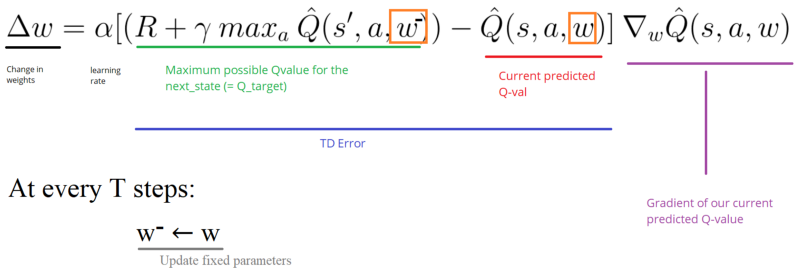
Fixed Q targets. The local network is learning values that a different target network has estimated. Therefore, the formula above is decoupled into the following:
  q_target(state, action, target_network) = discount * (reward + value(next_state, target_network))
  q_local = q_table(state, action)
  q_table(state, action) = q_local + alpha * (q_target - q_local)
The Bellman equations for this are as follows:
Riedmiller, Martin. "Neural fitted Q iteration–first experiences with a data efficient neural reinforcement learning method." European Conference on Machine Learning. Springer, Berlin, Heidelberg, 2005.
http://ml.informatik.uni-freiburg.de/former/_media/publications/rieecml05.pdf

Mnih, Volodymyr, et al. "Human-level control through deep reinforcement learning." Nature518.7540 (2015): 529.
http://www.davidqiu.com:8888/research/nature14236.pdf
With the two core concepts, deep-q-learning is able to play atari-games and solve this banana collection task!
The value estimation of the next state can be overestimated. This happens, because only the maximum q-value of each noisy action is used. The idea of Double Q-learning is to reduce overestimations by decomposing the max operation in the target into action selection and action evaluation. Although not fully decoupled, the target network in the DQN architecture provides a natural candidate for the second value function, without having to introduce additional networks. It is therefore proposed to evaluate the greedy policy according to the online network, but using the target network to estimate its value.
Prioritized experience replay gives priority to experiences with a big loss. These high-loss experiences get sampled for new learning more often. This introduced bias needs to be mitigated especially in the late stages of training. Therefore the paper suggests to compensate the bias by learning less fast from these high-loss samples. At the end of learning, this bias needs high or full compensation.
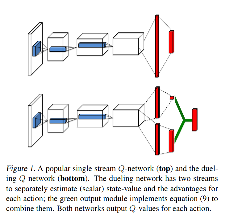
The core idea is to estimate state-value functions v(s) and the advantage of each action seperately and combine them into an output. The beauty of this algorithm is that it only changes the network architecture and can be combined neatly into the dqn architecture with addons.
    "We propose a conceptually simple and lightweight framework for deep reinforcement learning that uses
    asynchronous gradient descent for optimization of deep neural network controllers. We present asynchronous
    variants of four standard reinforcement learning algorithms and show that parallel actor-learners have a
    stabilizing effect on training allowing all four methods to successfully train neural network controllers.
    The best performing method, an asynchronous variant of actor-critic, surpasses the current state-of-the-art
    on the Atari domain while training for half the time on a single multi-core CPU instead of a GPU. Furthermore,
    we show that asynchronous actor-critic succeeds on a wide variety of continuous motor control problems as
    well as on a new task of navigating random 3D mazes using a visual input. "
    "In this paper we argue for the fundamental importance of the value distribution: the distribution of the random
    return received by a reinforcement learning agent. This is in contrast to the common approach to reinforcement
    learning which models the expectation of this return, or value. Although there is an established body of
    literature studying the value distribution, thus far it has always been used for a specific purpose such as
    implementing risk-aware behaviour. We begin with theoretical results in both the policy evaluation and control
    settings, exposing a significant distributional instability in the latter. We then use the distributional
    perspective to design a new algorithm which applies Bellman's equation to the learning of approximate value
    distributions. We evaluate our algorithm using the suite of games from the Arcade Learning Environment. We
    obtain both state-of-the-art results and anecdotal evidence demonstrating the importance of the value
    distribution in approximate reinforcement learning. Finally, we combine theoretical and empirical evidence to
    highlight the ways in which the value distribution impacts learning in the approximate setting."
    "We introduce NoisyNet, a deep reinforcement learning agent with parametric noise added to its weights, and
    show that the induced stochasticity of the agent's policy can be used to aid efficient exploration. The
    parameters of the noise are learned with gradient descent along with the remaining network weights. NoisyNet is
    straightforward to implement and adds little computational overhead. We find that replacing the conventional
    exploration heuristics for A3C, DQN and dueling agents (entropy reward and ϵ-greedy respectively) with
    NoisyNet yields substantially higher scores for a wide range of Atari games, in some cases advancing the
    agent from sub to super-human performance."
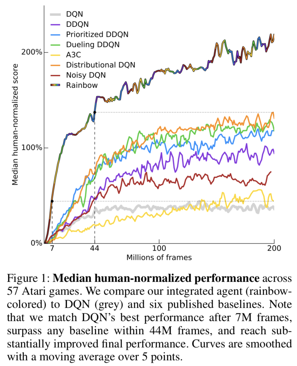
    "The deep reinforcement learning community has made several independent improvements to the DQN algorithm.
    However, it is unclear which of these extensions are complementary and can be fruitfully combined. This
    paper examines six extensions to the DQN algorithm and empirically studies their combination. Our experiments
    show that the combination provides state-of-the-art performance on the Atari 2600 benchmark, both in terms of
    data efficiency and final performance. We also provide results from a detailed ablation study that shows the
    contribution of each component to overall performance."
The components are further described in the blogpost
The repository contains the following algorithms with optimized parameters
- Vanilla DQN
- Double DQN
- Dueling DQN
- Prioritized experience replay with a Sum Tree Each algorithm can be switched off and on individually. To help understanding, the interested reader can search for the occurrence of these switches and learn about their effect on the overall DQN architecture.
The Double DQN uses a simple network architecture exhibiting fully connected layers. This simple architecture is suitable to learn the required Q_values without a lot of data. The dqn_model_test loads the dqn network and prints the nodes.
(fc1): Linear(in_features=37, out_features=64, bias=True) (fc2): Linear(in_features=64, out_features=64, bias=True) (fc3): Linear(in_features=64, out_features=4, bias=True) (state_value): Linear(in_features=64, out_features=1, bias=True)
The activation functions are relu and as Adam Optimizer was chosen.
The following parameters help the network to learn fast. It is interesting to note that the Epsilon decays faster and the learning rate is higher to boost fast learning of a relatively simple task.
The parameters from the Atari Papers work well. With the small network, a score of 13 is achieved in 550 episodes.
The parameters from the prioritized experience replay are:
Learning rate 1e-4, learn every 4 steps from 32 episodes. If the agent learns every 16 steps from 256 episodes, the
steps are fewer, but the episodes are faster due to the usage of a graphics card with enough memory.
The average score is improved from 14.3 to 15 in fewer episodes.
A faster training can be achieved using the following parameters:
Since the learning is quick, the experience buffer is smaller, because older examples do not represent the quickly adapted policy that well.
The network overfits beyond 700, indicated by reduced scores. The useful number of episodes varies greatly among the parameters. Basically if the network does not improve or substantially (more than 2 points from max) decreases, training is futile.
Only a small epsilon guarantuees high scores because the random parameters are typically non-optimal actions. Technically the skill of a learned agent should be evaluated with epsilon = 0.
- eps_start=1.0
- eps_min=0.01
- eps_decay=0.99
The batch size in combination with the update_every parameter shows how often experience is reused on average. In the current implementation 256 batch size does not cost a lot of extra time since the network is small. Learning at every 16 step means that the average experience is reused 8 times. The achievable score improves with bigger batches and faster learning events.
- BATCH_SIZE = 256 A large minibatch size stabilizes the learning parameters
- UPDATE_EVERY = 16 # how often to update the network
- BUFFER_SIZE = int(1e3) # replay buffer size
The discount factor gamma shows how far into the future the lookahead shows. The halftime of 0.99 is ~ 70 steps, so the agent roughly overlooks the entire episode of 300 steps weighing a step 2*70 ahead with 25 %.
- GAMMA = 0.99 The discount factor shows how much importance future expectand reward has
The soft update of the target parameters shows how far ahead the local network is from the target network. If this parameter is too big, it destabilizes learning.
- TAU = 1e-2 # for soft update of target parameters
Using double-dqn, a learning rate of 1e-3 is better, for prioritized experience replay 1e-4 is showing better results.
- LR = 1e-3 # learning rate.
Achieved score
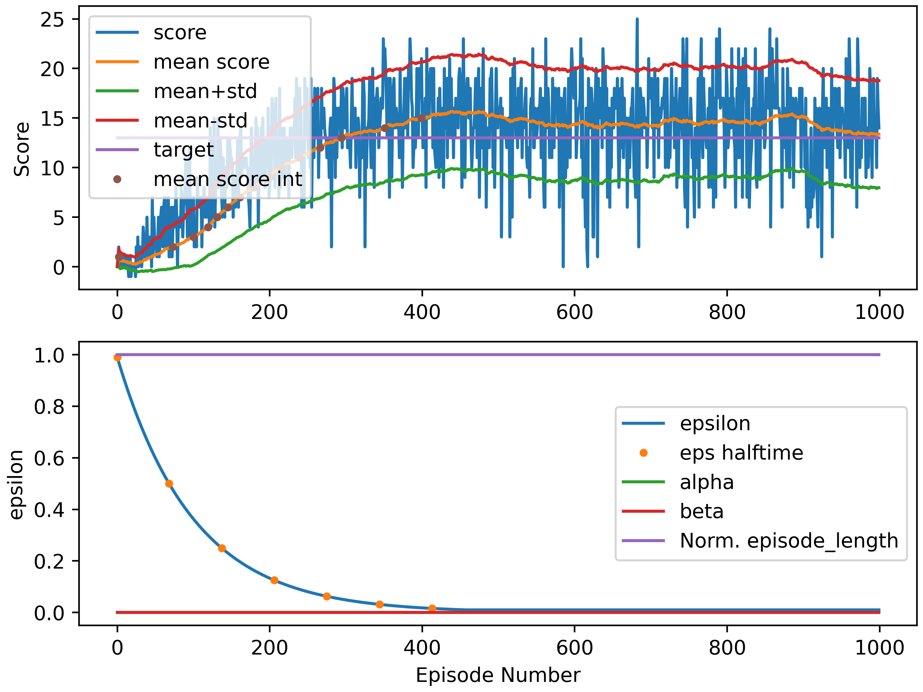
The environment is solved in ~300 episodes with an average score of 100 episodes above 13. After 400 Episodes, a score of 15 is achieved. This run uses double and dueling algorithms as well as the above parameters with a small 64, 64 neural network. The watch.py file uses the weights obtained at episode 400 of this run.
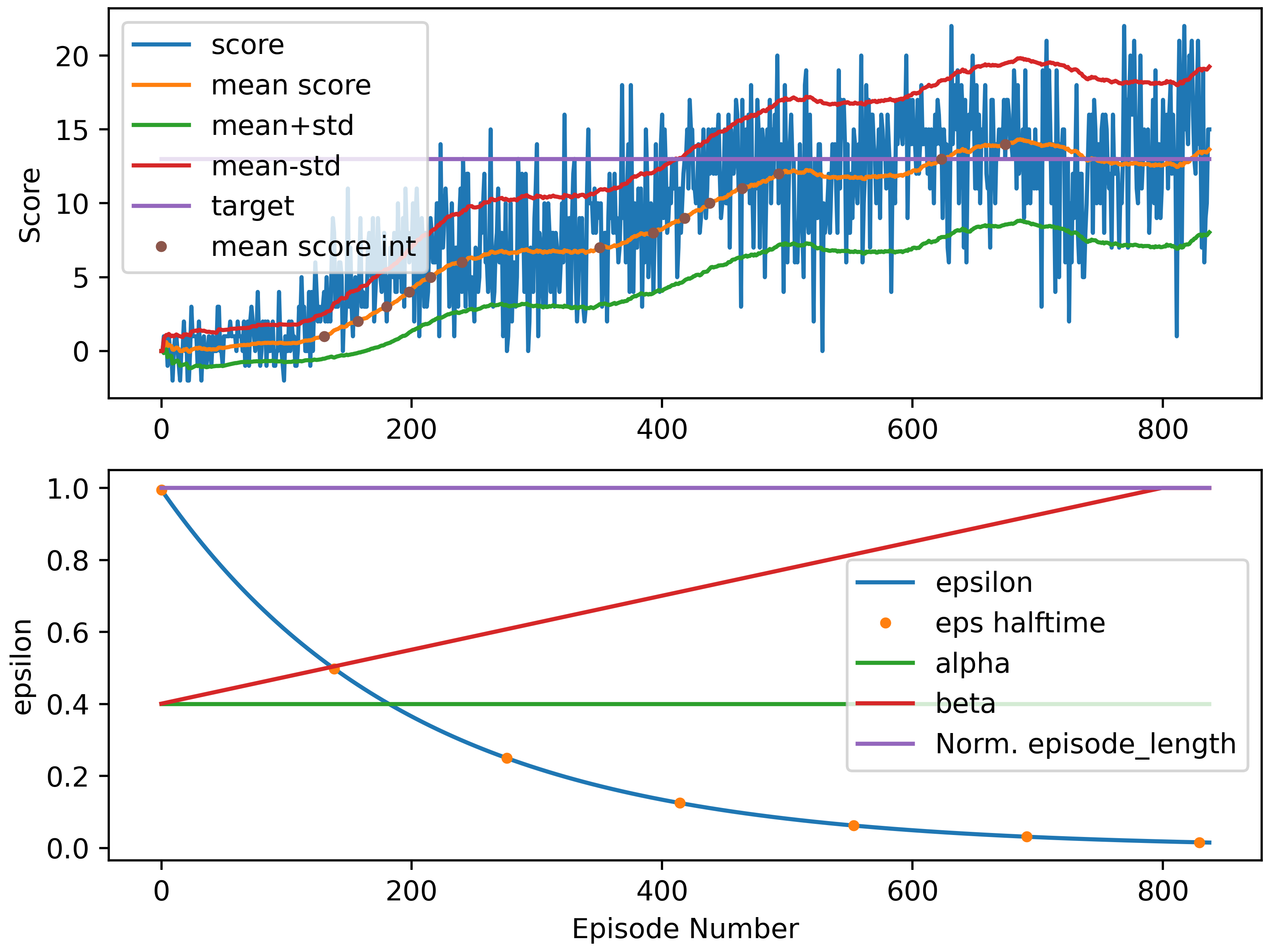
The best run using Prioritized experience Replay is shown in the following diagram. The weighting factors for using PER are 0.4 in order to achieve a high score. The learning rate is set to 1e-4 in contrast to the above implementation with 1e-3. The batch_size is increased to 512 and the experience buffer is tripled to 2^15 (a number beneficial for the sum tree).
Currently the policy search samples a trajectory based on the configured parameters in arguments.py. These arguments are randomly altered and a training trajectory is rolled out.
Hill climbing is an iterative algorithm that can be used to find the weights θ for an optimal policy. By slightly perturbing the values of the current best estimate for the weights θbest, a new set of weights is yielded. These new weights are then used to collect an episode. If the new weights θnew resulted in higher return than the old weights, then θnew is set as the new θbest.
Steepest ascent hill climbing is a variation of hill climbing that chooses a small number of neighboring policies at each iteration and chooses the best among them.
Simulated annealing uses a pre-defined schedule to control how the policy space is explored, and gradually reduces the search radius as we get closer to the optimal solution.
Adaptive noise scaling decreases the search radius with each iteration when a new best policy is found, and otherwise increases the search radius.
The trajectory gets rated according to max average score and the average score overall. This favors an algorithm that achieves a high score and learns fast. The best rated trajectory is modified randomly according to a predefined set of parameters to be sampled from. The idea stems from the PER paper, which gives reasonable ranges for parameters. The parameters are based on typical parameter ranges. For each step, the best known parameter set gets mutated.
In Hillclimbing, parameters get changed by a small offset. But this approach does not account for the parameters to be optimized here, which sometimes can vary in factors of 10 or 100. Therefore, two parameters get chosen and sampled randomly at each iteration to generate a new trajectory. Previously sampled trajectories get not rolled out again, because the computational burden is too high.
The cross-entropy method iteratively suggests a small number of neighboring policies, and uses a small percentage of the best performing policies to calculate a new estimate.
The evolution strategies technique considers the return corresponding to each candidate policy. The policy estimate at the next iteration is a weighted sum of all of the candidate policies, where policies that got higher return are given higher weight.
Each run gets logged with an matplotlib-diagram, a csv and a yaml. The image shows the learnign progress in a representative way. The csv and yaml show similar data, but sometimes a quick look into a csv spreadsheet is nice. The logged data also show the trajectories of characteristic values to allow for post-analysis in detail.
Currently, the alternated parameters are: 'learning_rate', 'fc1', 'fc2', 'annihilation_lengths', 'alpha', 'beta_start', 'batch_size', 'epsilon_decay', 'tau', 'update_every', 'per_eps', 'buffer_size'
Then, it would be very interesting to use saliency maps and the visual simulator to further analyze the algorithmic performance and fallacies.
Watching the agent, a more capable neural network could improve the behavior in the environment.
unityagents.exception.UnityEnvironmentException: Couldn't launch the Banana environment. Provided filename does not match any environments.
means the unityenvironment is not found. The path is configured in dqn/arguments.py in line 12. Using linux, the downloaded folder should be placed in this root directory.

