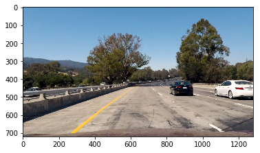
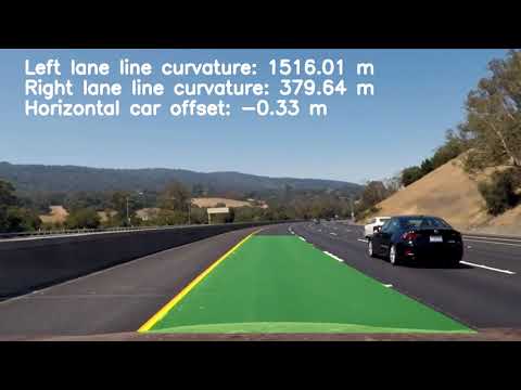
The goals / steps of this project are the following:
- Compute the camera calibration matrix and distortion coefficients given a set of chessboard images.
- Apply a distortion correction to raw images.
- Use color transforms, gradients, etc., to create a thresholded binary image.
- Apply a perspective transform to rectify binary image ("birds-eye view").
- Detect lane pixels and fit to find the lane boundary.
- Determine the curvature of the lane and vehicle position with respect to center.
- Warp the detected lane boundaries back onto the original image.
- Output visual display of the lane boundaries and numerical estimation of lane curvature and vehicle position.
I have defined the camera_calibration function which takes as input parameters an array of paths to chessboards images, and the number of inside corners in the x and y axis.
The function is located in calibration.py.
For each image path, calibrate_camera:
- reads the image by using the OpenCV cv2.imread function,
- converts it to grayscale usign cv2.cvtColor,
- find the chessboard corners usign cv2.findChessboardCorners
- Finally, the function uses all the chessboard corners to calibrate the camera by invoking cv2.calibrateCamera.
Here is how I used my function:
mtx, dist = calibration.camera_calibration(images, 6, 9)I have then used the returned camera matrix and distortion coefficients from my camera_calibration function to perform a distortion correction on a chessboard image.
Here is how I used it and output images:
img = cv2.imread('./camera_cal/calibration1.jpg')
undistorted_img = cv2.undistort(img, mtx, dist, None, mtx)

helpers.plt_images(img, 'Source image', undistorted_img, 'Undistorted image')In order to create the final binary image I've create a treshold.py file containing needed funtions to calculate several gradient measurements (x, y, magnitude, direction and color).
- Calculate directional gradient: abs_sobel_thresh().
- Calculate gradient magnitude: mag_thresh().
- Calculate gradient direction: dir_threshold().
- Calculate color threshold: col_thresh().
- Then, combine_threshs() will be used to combine these thresholds, and produce the image which will be used to identify        lane lines in later steps.
Here is how I used these functions and their respective outputs:
<matplotlib.image.AxesImage at 0x102f994a8>
grad_x = threshold.abs_sobel_thresh(image, orient='x', thresh=(30, 100))
helpers.plt_images(image, 'Source image', grad_x, 'Directional gradient')
grad_y = threshold.abs_sobel_thresh(image, orient='y', thresh=(30, 100))
helpers.plt_images(image, 'Source image', grad_y, 'Directional gradient')mag_binary = threshold.mag_thresh(image, sobel_kernel=3, thresh=(70, 100))
helpers.plt_images(image, 'Source image', mag_binary, 'Gradient magnitude')dir_binary = threshold.dir_threshold(image, sobel_kernel=15, thresh=(0.7, 1.3))
helpers.plt_images(image, 'Source image', dir_binary, 'Gradient direction')col_binary = threshold.col_thresh(image, thresh=(170, 255))
helpers.plt_images(image, 'Source image', col_binary, 'Gradient direction')combined = threshold.combine_threshs(grad_x, grad_y, mag_binary, dir_binary, col_binary, ksize=15)
helpers.plt_images(image, 'Source image', combined, 'Combined thresholds')I've create a warp.py file containing needed funtions to apply a perspective transform to rectify binary image ("birds-eye view"). The complete process I followed to can be described like this:
- Select the coordinates corresponding to a trapezoid in the image.
- Define the destination coordinates, or how that trapezoid would look from birds_eye view.
- Use function cv2.getPerspectiveTransform to calculate both, the perpective transform M and the inverse perpective transform _Minv.
M and Minv will then be used to warp and unwarp the video images.
Here is how I used my function and the output:
src_coordinates = np.float32(
    [[280,  700],  # Bottom left
     [595,  460],  # Top left
     [725,  460],  # Top right
     [1125, 700]]) # Bottom right

dst_coordinates = np.float32(
    [[250,  720],  # Bottom left
     [250,    0],  # Top left
     [1065,   0],  # Top right
     [1065, 720]]) # Bottom right

warped_img, _ , Minv  = warp.warp(image, src_coordinates, dst_coordinates)
# Visualize undirstorsion
f, (ax1, ax2) = plt.subplots(1, 2, figsize=(20,10))
ax1.set_title('Undistorted image with source points drawn', fontsize=16)
ax1.plot(Polygon(src_coordinates).get_xy()[:, 0], Polygon(src_coordinates).get_xy()[:, 1], color='red')
ax1.imshow(image)

ax2.set_title('Warped image with destination points drawn', fontsize=16)
ax2.plot(Polygon(dst_coordinates).get_xy()[:, 0], Polygon(dst_coordinates).get_xy()[:, 1], color='red')
ax2.imshow(warped_img)
<matplotlib.image.AxesImage at 0x102e68470>
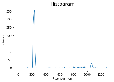
I have then created an histogram of the lower half of the warped image. The function used can be find in the helpers.py file.
Here is how I used it and the output:
# Run de function over the combined warped image
combined_warped = warp.warp(combined)[0]
histogram = helpers.get_histogram(combined_warped)

# Plot the results
plt.title('Histogram', fontsize=16)
plt.xlabel('Pixel position')
plt.ylabel('Counts')
plt.plot(histogram)
[<matplotlib.lines.Line2D at 0x102c0a5c0>]
The next step is to use Sliding Window technique to identify the most likely coordinates of the lane lines in a window. For that I've created lines.py file with the needed function. The process to detect the lines can be explained as follow:
- The starting left and right lanes positions are selected by looking to the max value of the histogram to the left and the right of the histogram's mid position.
- Sliding Window is used to identify the most likely coordinates of the lane lines in a window, which slides vertically through the image for both the left and right line.
- Then usign the coordinates previously calculated, a second order polynomial is calculated for both the left and right lane line using Numpy's function np.polyfit.
Here is how I used the function and the output
lines_fit, left_points, right_points, out_img = lines.detect_lines(combined_warped, return_img=True)
helpers.plt_images(warped_img, 'Warped image', out_img, 'Lane lines detected')I have then create detect_similar_lines() that uses the previosly calculated line_fits to try to identify the lane lines in a consecutive image.
Here is how I used the function and the output:
lines_fit, left_points, right_points, out_img = lines.detect_similar_lines(combined_warped, lines_fit, return_img=True)
helpers.plt_images(warped_img, 'Warped image', out_img, 'Lane lines detected')
Clipping input data to the valid range for imshow with RGB data ([0..1] for floats or [0..255] for integers).
I have then calculated the curvature radius and the car offset using two functions that can be find in the lines.py file
to calculate the curvature radius: - Fit a second order polynomial to pixel positions in each fake lane line - Define conversions in x and y from pixels space to meters - Fit new polynomials to x,y in world space - Calculate the new radius of curvature - return the new radius of curvature in meters
Here is how the function is used and the output:
curvature_rads = lines.curvature_radius(leftx=left_points[0], rightx=right_points[0], img_shape = img.shape)
print('Left line curvature:', curvature_rads[0], 'm')
print('Right line curvature:', curvature_rads[1], 'm')
Left line curvature: 518.4476261684651 m
Right line curvature: 1558.810189537155 m
Here is how the car offset function is used and the output:
offsetx = lines.car_offset(leftx=left_points[0], rightx=right_points[0], img_shape=img.shape)
print ('Car offset from center:', offsetx, 'm.')
Car offset from center: -0.0560041662700661 m.
Then I've drawn the lines onto the image. For this purpose I've created a file called draw.py
- Draw the lane lines onto the warped blank version of the image.
- Warped back to original image space using inverse perspective matrix (Minv).
Here is how I used the function and the output:
img_lane = draw.draw_lane(image, combined_warped, left_points, right_points, Minv)
helpers.plt_images(image, 'Test image', img_lane, 'Lane detected')I have then added metrics onto this image using the add_metrics function in draw.py
Here is how the function is used and the output:
out_img = draw.add_metrics(img_lane, leftx=left_points[0], rightx=right_points[0])
helpers.plt_images(image, 'Test image', out_img, 'Lane detected with metrics')
Output visual display of the lane boundaries and numerical estimation of lane curvature and vehicle position video
And finally I have used all the above to create a Pipeline class that can be used on a video. You can find the class in the notebook where all the code is written: advance_line_finding.ipynb
-
Improvement:
- Smoothing: Each time a new high-confidence measurement is calculated, it can be appended to the list of recent measurements and then take an average over n past measurements to obtain the lane position to draw onto the image.
-
Likely to fail:
- White cars: There is a possibility I think where the pipeline could if a white car is too close in front of us.


