specieshindex is a package that aims to gauge scientific influence of
different species (or higher taxa) mainly using the h-index.
To get this package to work, make sure you have the following packages installed.
remotes::install_github("jessicatytam/specieshindex", build_vignettes = TRUE, dependencies = TRUE)

#Load the library
library(specieshindex)

#See the vignette
vignette("specieshindex")Functions that extract data will only run if you or your institution are a paid subscriber. Make sure you are connected to the internet via institutional access or acquire a VPN from your institution if you are working from home. Alternatively, if you are a subscriber of Scopus already, you can ignore this step.
To connect and download citation information from Scopus legally, you will absolutely need an API key. Here are the steps to obtain the key.
- Go to https://dev.elsevier.com/ and click on the button
I want an API key. - Create an account and log in.
- Go to the
My API Keytab on top of the page and clickCreate API Key. - Read the legal documents and check the boxes.
After acquiring your key, make sure to store it safely. The following steps will enable you to save it as an environment variable, without saving it in the console or script.
file.edit("~/.Renviron")This will bring up an empty file, which is where you will save your key into.
Elsevier_API = "a_long_string"Restart your session for this to work. To retrieve your key, use
Sys.getenv():
Sys.getenv("Elsevier_API")
#> [1] "a_long_string"
You can then load it to your environment as follows:
apikey <- Sys.getenv("Elsevier_API")You are required to be at your institution for this to work since the API is accessed via the IP address. Run the following line of code to do so:
sid <- auth(username = NULL, password = NULL)You won’t have to set this again until your next session. You are required to be at your institution for this to work since the API is accessed via the IP address.
You must have your IP address whitelisted. You can do it here.
Here is a quick demonstration of how the package works.
Multiple databases have been incorporated into specieshindex, namely
Scopus, Web of Science, and BASE. To differentiate between them, set the
db parameter to your desired database. You can set search = "t" for
search terms in the title only and search = "tak" for search terms in
the title, abstract, or keywords. For genus-level searches, leave the
species parameter empty. If you are only interested in knowing how
many publications there are, you can run the Count() functions.
#Title only; species level
Count(db = "scopus",
      search = "t",
      genus = "Bettongia", species = "penicillata")

#Title, abstract, or keywords; genus level
Count(db = "scopus",
      search = "tak",
genus = "Bettongia")In order to calculate the indices, you will need to download the
citation records. The parameters of Count() and Fetch() are exactly
the same. Let’s say you want to compare the species h-index of a few
marsupials. First, you would need to download the citation information
using Fetch(). Remember to use binomial names.
Woylie <- Fetch(db = "scopus",
                search = "tak",
                genus = "Bettongia", species = "penicillata")
Quokka <- Fetch(db = "scopus",
                search = "tak",
                genus = "Setonix", species = "brachyurus")
Platypus <- Fetch(db = "scopus",
                  search = "tak",
                  genus = "Ornithorhynchus", species = "anatinus")
Koala <- Fetch(db = "scopus",
               search = "tak",
genus = "Phascolarctos", species = "cinereus")The Count() and Fetch() functions allow the addition of keywords
using Boolean operators to restrict the domain of the search. Although
you can simply use keywords such as “conservation”, you will find that
using “conserv*” will yield more results. The “*” (or wildcard) used
here searches for any words with the prefix “conserv”,
e.g. conservation, conserve, conservatory, etc. Find out more about
search language
here and
here.
Some species have had their classification changed in the past, resulting in multiple binomial names and synonyms. Synonyms can be added to the search strings to get the maximum hits. If you have more than 1 synonym, you can parse a list (the list should be named “synonyms”) into the argument.
Now that you have the data, you can use the Allindices() function to
create a dataframe that shows their indices.
#Calculate indices
W <- Allindices(Woylie,
                genus = "Bettongia", species = "penicillata")
Q <- Allindices(Quokka,
                genus = "Setonix", species = "brachyurus")
P <- Allindices(Platypus,
                genus = "Ornithorhynchus", species = "anatinus")
K <- Allindices(Koala,
                genus = "Phascolarctos", species = "cinereus")

CombineSp <- dplyr::bind_rows(W, Q, P, K) #combining the citation records
CombineSp
#>              genus_species     species           genus publications citations
#> 1    Bettongia penicillata penicillata       Bettongia          113      1903
#> 2       Setonix brachyurus  brachyurus         Setonix          242      3427
#> 3 Ornithorhynchus anatinus    anatinus Ornithorhynchus          321      6365
#> 4   Phascolarctos cinereus    cinereus   Phascolarctos          773     14291
#>   journals years_publishing  h     m i10 h5
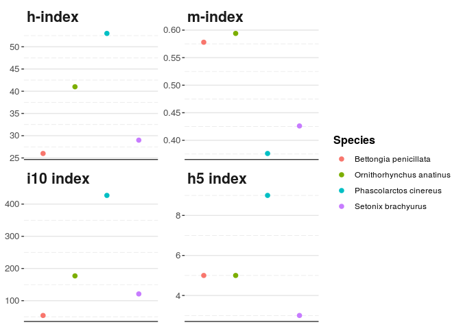
#> 1       55               45 26 0.578  54  5
#> 2      107               68 29 0.426 121  3
#> 3      153               69 41 0.594 177  5
#> 4      227              141 53 0.376 427  9
Once you are happy with your dataset, you can make some nice plots.
Using plotAllindices(), we can compare the indices against each other.
plotAllindices(CombineSp)Figure 1. The h-index, m-index, i10 index, and h5 index of the Woylie, Platypus, Koala, and Quokka.
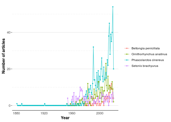
You can also visualise the total publication per year with getYear()
and plotPub().
extract_year_W <- getYear(data = Woylie,
                          genus = "Bettongia", species = "penicillata")
extract_year_Q <- getYear(data = Quokka,
                          genus = "Setonix", species = "brachyurus")
extract_year_P <- getYear(data = Platypus,
                          genus = "Ornithorhynchus", species = "anatinus")
extract_year_K <- getYear(data = Koala,
                          genus = "Phascolarctos", species = "cinereus")
Combine_pub <- rbind(extract_year_W, extract_year_Q, extract_year_P, extract_year_K)
plotPub(Combine_pub)
Figure 2. The total number of publications per year of the Woylie, Platypus, Koala, and Quokka.
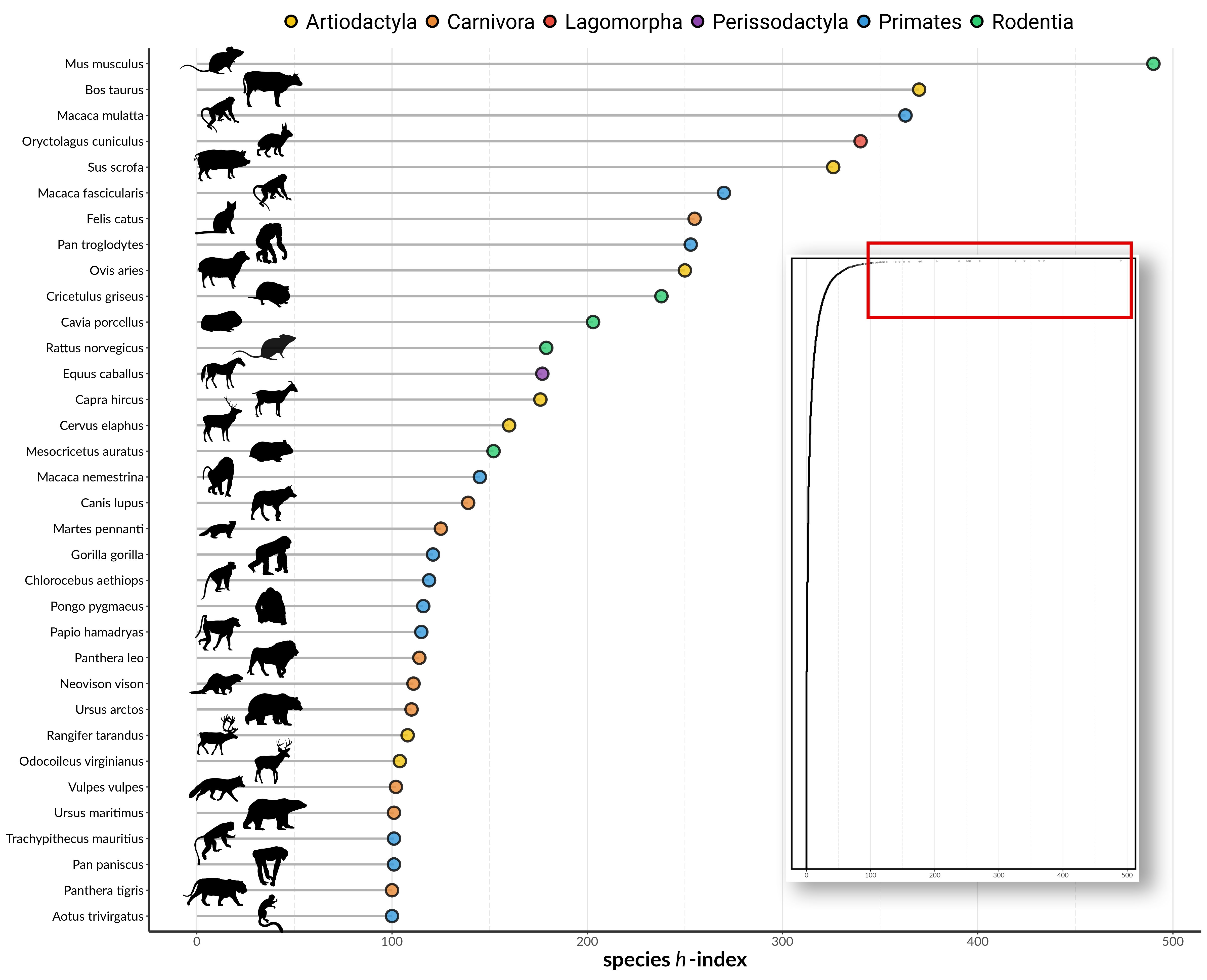
To see a concrete example, Tam et al. (2021) has applied this package to study taxonomic bias among mammals by quantifying the scientific interest of 7,521 species of mammals.
Figure 3. Species h-index of mammals with a species h-index of h = 100 and larger (adapted from Tam et al. (2021)).
specieshindex is enabled by Scopus, Web of Science, and BASE.
To propose any bug fixes or new features, please refer to our community guidelines.


