This code uses the algebra solver in Stan to find the parameters of a distribution that produce a desired tail behavior. This can be a useful tool when choosing parameters for prior distributions. Here’s how to use it:
- Choose a distribution.
- Define the quantile boundaries and the amount of probability density that you wish to have above and below those boundaries.
- Let Stan go find the parameters that produce the desired distribution.
Currently supported distributions:
- Normal
- Log-Normal
- Beta
- Gamma
- Inverse Gamma
Obviously you need to have Stan installed on your machine.
If you don’t want to use the shiny app interface, you only need to have
the rstan library installed:
install.packages('rstan')To use the shiny app, you will also need to install the shiny and
shinycssloaders libraries:
install.packages('shiny')
install.packages('shinycssloaders')To use the Shiny app, just run the following code in R:
library(shiny)
runGitHub('jhelvy/stanTuneR')
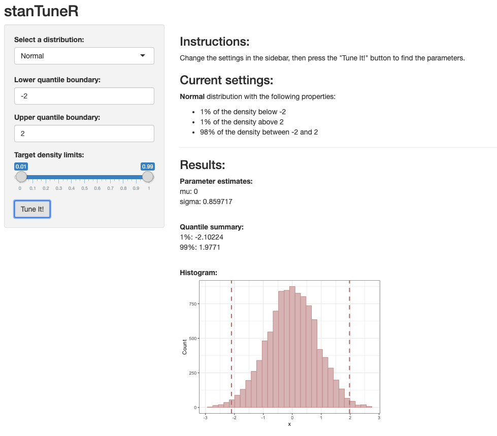
The interface should look like this:
(see the examples.R file for more examples)
Let’s say I want to find the parameters of a normal distribution such that P[x < -2.0] ~ 0.01 and P[x > 2.0] ~ 0.01. That is, I want a normal distribution where 98% of the probability density is between (-2, 2).
First, load the rstan library, tweak some settings, and source the
functions.R file (all functions are loaded in a new environment called
funcs):
# Load libraries
library(shiny)
library(rstan)

# Stan settings
rstan_options(auto_write = TRUE)
options(mc.cores = parallel::detectCores())

# Load the functions
funcs <- new.env()
source('functions.R', local=funcs)
Then use the targets argument to set the desired tail properties:
targets = list(
    bound_L = -2,   # LOWER quantile boundary
    bound_U = 2,    # UPPER quantile boundary
    dens_L  = 0.01, # Target density below LOWER quantile boundary
    dens_U  = 0.01) # Target density above UPPER quantile boundary
Then use the tuneParams function to find the parameters:
results = funcs$tuneParams(distribution='normal', targets)##
## SAMPLING FOR MODEL 'model' NOW (CHAIN 1).
## Chain 1: Iteration: 1 / 1 [100%] (Sampling)
## Chain 1:
## Chain 1: Elapsed Time: 0 seconds (Warm-up)
## Chain 1: 0.001128 seconds (Sampling)
## Chain 1: 0.001128 seconds (Total)
## Chain 1:
View the resulting parameters and verify that the quantiles of 10,000 draws from the resulting distribution match your criteria:
results$params## $mu
## [1] 0
##
## $sigma
## [1] 0.859717
results$quantiles## 1% 99%
## -2.027173 2.066950
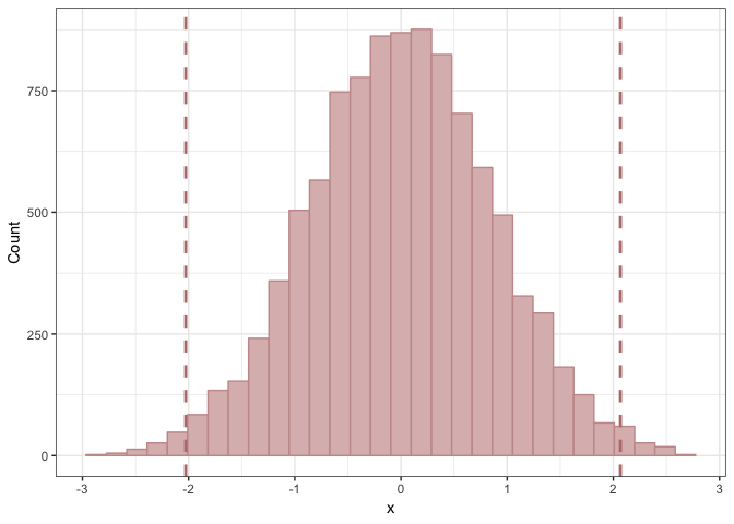
Finally, view a histogram of the resulting distribution:
results$histogramThe meat of this app is in the functions.R code. The main function is
the tuneParams() function. After the user defines the distribution
and the targets for the quantiles and density, tuneParams() calls
the generateStanCode() function to generate the Stan code for the
model, which is written to the file model.stan. This file is always
overwritten every time the generateStanCode() function is called. It
then calls the stan function to fit the model. Finally, once the model
is fit, it calls the summarizeResults() function to extract the
results of the fit model. The output of tuneParams() is a list with
the following values:
params: The fit parametersdraws: 10,000 draws from the resulting distribution using the fit parametersquantiles: The quantiles of the draws at the desired upper and lower quantile boundarieshistogram: A histogram of the draws
- Author: John Paul Helveston (www.jhelvy.com)
- Date First Written: Tuesday, April 30, 2019
- License: GPL-3

