Run this to compute taxonomic outliers within datasets on GBIF. This method uses vegan::taxa2dist to compute taxonomic distances.
Run on c4 or c5 something like that.
spark2-shell
import org.apache.spark.sql.functions._
val sqlContext = new org.apache.spark.sql.SQLContext(sc)

// val D = sqlContext.sql("SELECT * FROM uat.occurrence_hdfs").
val D = sqlContext.sql("SELECT * FROM prod_h.occurrence_hdfs").
select("datasetkey","kingdomkey","phylumkey","orderkey","classkey","familykey","genuskey").
groupBy("datasetkey","kingdomkey","phylumkey","orderkey","classkey","familykey","genuskey").
agg(count(lit(1)).alias("num_of_occ")).
sort($"datasetkey",$"kingdomkey".desc,$"num_of_occ".desc);

import org.apache.spark.sql.DataFrame;

val make_external_table = (df: DataFrame, tableName: String) => {
df.createOrReplaceTempView(tableName + "_temp");
val x = df.columns.toSeq.mkString(" STRING, ");
val create_sql = "CREATE EXTERNAL TABLE jwaller." + tableName + " (" + x + " STRING) ROW FORMAT DELIMITED FIELDS TERMINATED BY '\t' STORED AS TEXTFILE LOCATION '/user/jwaller/" + tableName + ".csv'";
val overwrite_sql = "INSERT OVERWRITE TABLE jwaller." + tableName + " SELECT * FROM " + tableName + "_temp";

println(create_sql);
println(overwrite_sql);

sqlContext.sql(create_sql);
sqlContext.sql(overwrite_sql);
sqlContext.sql("show tables from jwaller").show(100);
}

make_external_table(D,"dataset_taxonkey_counts");
hdfs dfs -getmerge /user/jwaller/dataset_taxonkey_counts.csv dataset_taxonkey_counts.tsv
sed -i 's#\\N##g' dataset_taxonkey_counts.tsv
sed -i '1i datasetkey\tkingdomkey\tphylumkey\torderkey\tclasskey\tfamilykey\tgenuskey\tnum_of_occ' dataset_taxonkey_counts.tsv

// scp -r jwaller@c4gateway-vh.gbif.org:/home/jwaller/ /cygdrive/c/Users/ftw712/Desktop/jwaller/
// scp -r jwaller@c5gateway-vh.gbif.org:/home/jwaller/ /cygdrive/c/Users/ftw712/Desktop/jwaller/
library(dplyr)
library(roperators)
library(dplyr)
library(purrr)

file = "C:/Users/ftw712/Desktop/taxon_outliers/data/dataset_taxonkey_counts.tsv"

gbifTaxonOutliers::outlier_data_for_dataset_taxonkey_counts(file) %>%
saveRDS(file="C:/Users/ftw712/Desktop/outlier_data.rda")
outlier_data.rda will be a data.frame with the following columns.
- variable: a unique taxonkey in the dataset (usually at the rank of species). Can be rank family if dataset has more than 10K unique species because the distance matrix becomes very large.
- row_dist: the mean taxonomic distance from all other taxa in the dataset.
- sd_row_dist: standard deviation of row_dist.
- mean_row_dist: the mean row_dist for the entire dataset (should be a single value repeated).
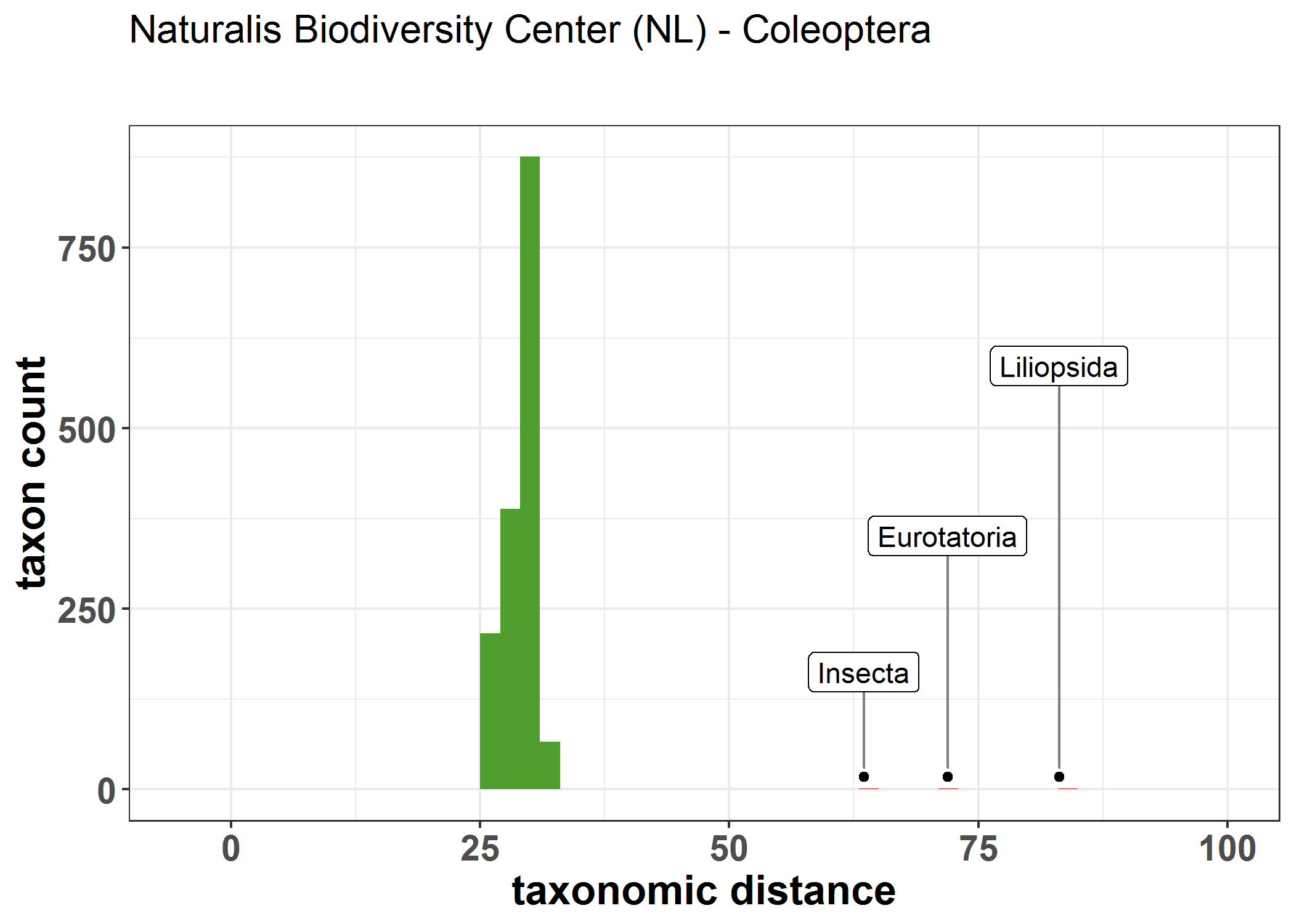
- outlier: the number of standard deviations away from the mean_row_dist. Values over 4 have been manually shown as good at flagging interpretation errors.
- datasetkey: the datasetkey for the dataset
Taxonomic distance here is normalized so as to be between 0 - 100. Roughly I think it works by dividing up the number of ranks into a distance divided by 100. So 4 rank levels would mean that the each rank would mean that 25% would be the minimum distance step. For example, if all taxa were in the same family, we would see that mean_row_dist would be around 25%. Datasets that are more diverse will have a larger value of sd_row_dist.
library(dplyr)
library(roperators)
library(dplyr)
library(purrr)

D = readRDS(file="C:/Users/ftw712/Desktop/outlier_data.rda") %>%
rename(taxon_key = variable) %>%
filter(datasetkey == "cca13f2c-0d2c-4c2f-93b9-4446c0cc1629") %>%
mutate(outlier = row_dist >= mean_row_dist + 4*sd_row_dist) %>%
glimpse()

point_data = D %>%
filter(outlier) %>%
gbifapi::addTaxonInfo(taxon_key) %>%
gbifapi::addDatasetTitle(datasetkey) %>%
glimpse()

library(ggplot2)

p = ggplot(D, aes(row_dist)) +
geom_histogram(binwidth = 2,aes(fill = outlier))

max_bin_height = ggplot_build(p)$data[[1]]$y %>% max()

p = p + theme_bw() +
scale_fill_manual(values = c("#509E2F", "red")) +
xlim(-5,100) +
theme(legend.position = "none")  +
ylab("taxon count") +
xlab("taxonomic distance") +
geom_point(data=point_data,aes(row_dist,y=max_bin_height*0.02)) +
ggrepel::geom_label_repel(
data=point_data,aes(row_dist,y=max_bin_height*0.02,label = class),
box.padding=3,
point.padding = 0.5,
segment.color = 'grey50',
direction = "y") +
ggtitle(unique(point_data$datasettitle)) +
theme(plot.title = element_text(family = "sans", size = 15, margin=margin(0,0,30,0))) +
theme(
axis.title.x = element_text(size = 16,face="bold"),
axis.title.y = element_text(size = 16,face="bold"),
axis.text.y = element_text(size = 14,face="bold"),
axis.text.x = element_text(size = 14,face="bold"),
)

ggsave("C:/Users/ftw712/Desktop/plot.pdf",plot=p)
googlesheet of potential errors: https://docs.google.com/spreadsheets/d/1waf8Gn9y35USmgeqDycCml3AnTdsIWaMJvYdMl4ryxM/edit#gid=275698222