Training a neural network to act as a surrogate model for Agent Based Models to speed up the simulation of mechanistic models used in the Das Lab.
Here's a very quickly put together set of slides that provides some background and that generally summarizes the work being attempted.
Here's a compilation of slides that contain figures that are related but also poorly organized.
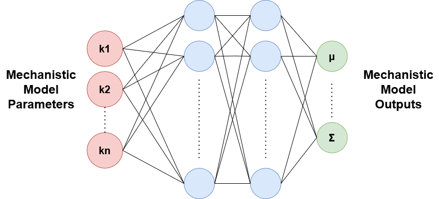
Simply put, surrogate modeling is when one designs a "surrogate" model, usually with some black-box method, that sufficiently approximates the behavior of a pre-existing model. Generally, speaking, surrogate models approximate models with some "mechanistic" or interpretable behavior such that its fast computations are of something meaningful. In this repository, we explore various different deep learning architectures for surrogate modeling. In particular, we take inspiration from the following paper here where a mapping is formed between cellular automata model parameters and its corresponding outputs.
However, there exists many other approaches where some are more suitable than others. A review of surrogate modeling for finite element method computations can be found here.
The big question one might ask is why create another model that models a model? While this seems like a very unnecessary roundabout step, especially when one considers the extra error in predictions resulting from adding an additional layer of abstraction, its speed benefits can not be neglected. See below for a quick example on the computational time needed to perform numerous simulations given a biochemical reaction model and its surrogate model.
| Nonlinear 6 Protein Model | Surrogate Model | |
|---|---|---|
| Number of Evaluations | 7,500 | 2,344 |
| Time (s) | 230 | 0.104 |
The surrogate model was approximately 691 times faster than the original model. The surrogate model is capable of scaling up to far larger numbers of evaluations, which is commonly needed when performing parameter estimation and identification (which is just another way of saying optimization or fitting) tasks. For reference, the actual model was evaluated in parallel on a 30-core CPU on a high performance compute cluster whereas the surrogate model was ran on my laptop GPU, one a vastly cheaper compute platform.
Here is a flowchart providing some contextual relationships as to how a surrogate relates to an actual mechanistic model and what we are using it for.
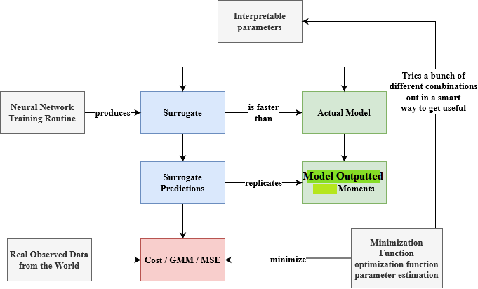
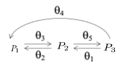
We started with a simple reaction network of a linear 3 protein model shown below,
In this case, the reaction network contained 5 sets of reactions (each with their own reaction rates, the thetas) and 3 abundances values (P1, P2, and P3). Given some set of 5,000 initial conditions of 3 proteins, a new set of 5,000 final conditions of 3 proteins are simulated. Taking these final conditions, we can derive some vector of 9 moments (means, variances, and covariances) of the final conditions at some time t. We do these moment computations, because there exists intrinsic noise from the reaction network simulation (i.e Gillespie) and the extrinsic noise resulting from the set of initial conditions. While this toy problem, once examined, is quite simple (as it can be approximated by a system of linear ODEs), it provided a useful frame of reference for this surrogate modeling project, because it incorporates some of the aspects that one might encounter when performing biological simulations (namely noise).
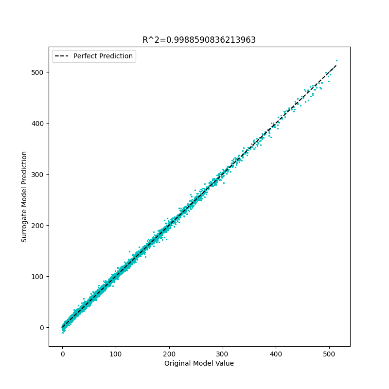
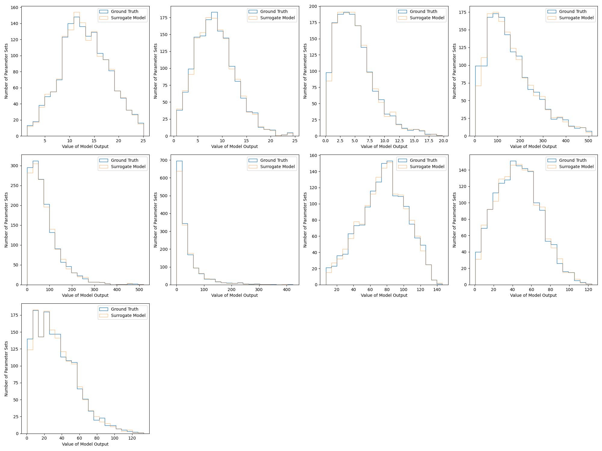
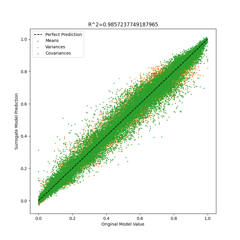
And, so, when training the surrogate model on some 8,500 sets of parameter sets to moment pairs, and then evaluating on 1,500 parameter sets in the test set, we get something that looks like this with a relatively low test average MSE of 0.0301 (please note that the abundance values range on the order of magnitude of 10^2) and an r^2 plot as well as histogram that looks like the figures below. Note that each histogram plot corresponds to some type of moment (E(X), E(X^2) E(XY), etc.).
Note: One should in principle do cross validation MSE loss (or some other metric) to get a better idea of how the surrogate model is truly performing (on average), but in this case, even with cross-validation, negligible generalization performance gains were seen (probably because the dataset contained a large number of parameter sets were sampled from some uniform distribution and thus were evenly spread out).
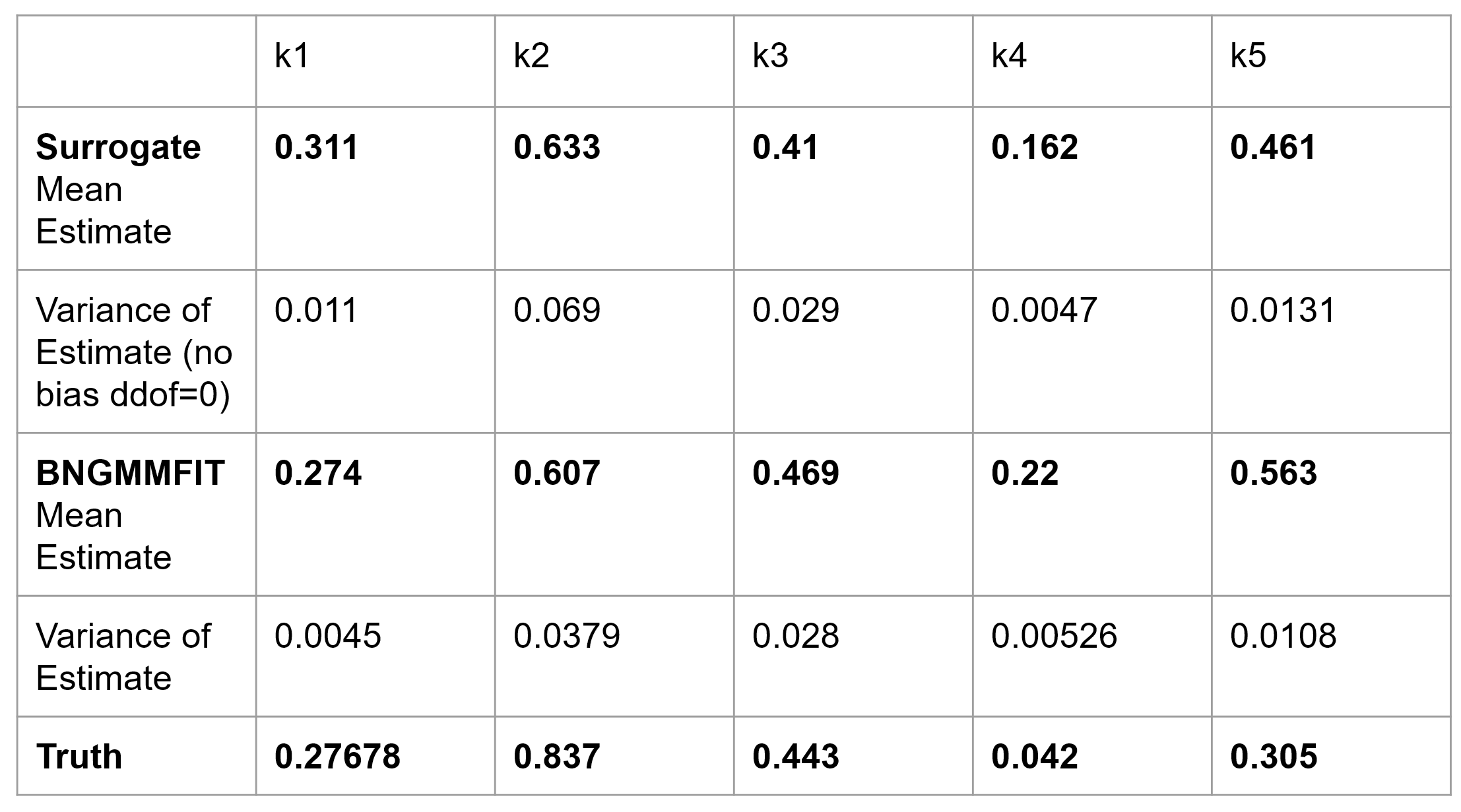
However, these plots while a useful litmus test, are not perfect. A better validation test is performing a parameter estimation task where one attempts to fit the surrogate model (and the actual model) to synthetically generated data with ground truth (as one would with real data). In this toy problem, we used particle swarm optimization to fit some synthetic observed data and we get the following parameter estimates.
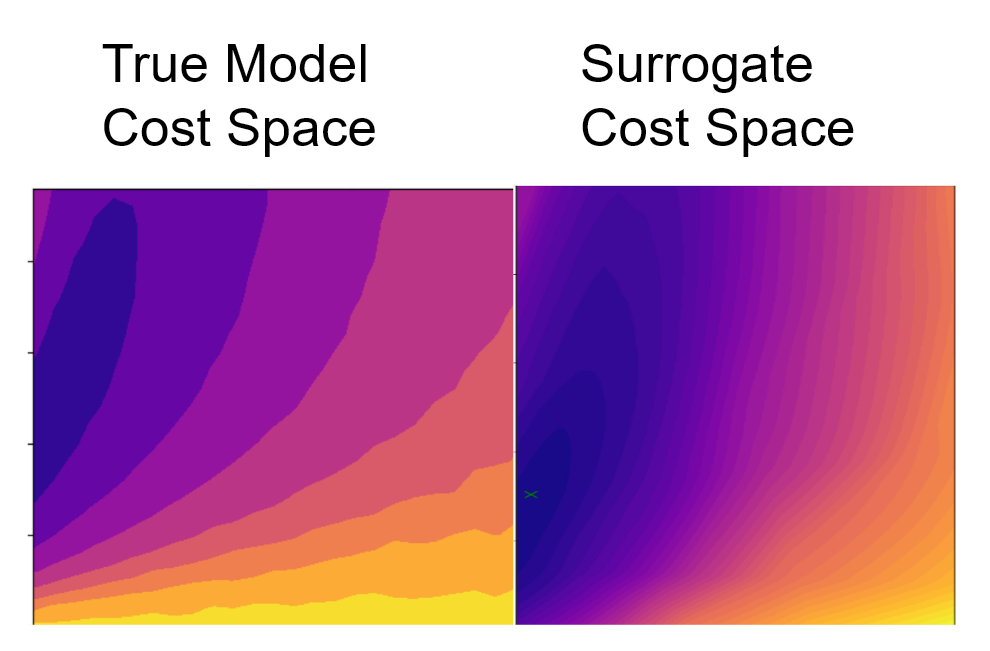
Furthermore, when creating cost contour plots where all thetas (or k's) are held constant at the simulated ground truth except for theta 4 and theta 5, one can observe that the mechanistic model's cost space is actually being well approximated by the surrogate.
Please note that because running the true model is often more computationally expensive than the surrogate model, the cost contour of the true model is lower resolution. On the other hand, the surrogate contour cost space is much higher resolution due to its fast speed of computation. However, even so, the shapes of the cost contour functions within the parameter space of theta 4 vs. theta 5 are of similar shape. Furthermore, the darker shaded regions indicating lower cost surround the ground truth parameters.
I had a highschooler do some experiments with different combinations of numbers of hidden neurons and layers in the deep surrogate models we've used for the linear 3 protein model. The results can be found here (Thanks Soham!). Unfortunately, the only general advice I can give is that larger neural networks are required for more complex mechanistic models where nonlinearity is often present. The exact numbers of layers, neurons, and even architecture is heavily problem specific.
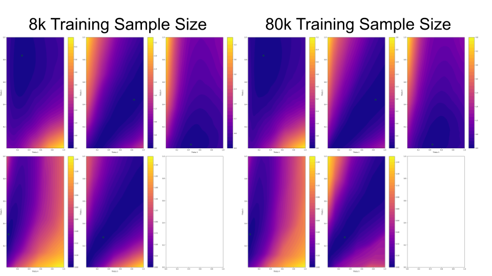
Similarly, dataset size is also equally problem specific. Depending on the behavior and parameter sensitivity in the mechanistic model, the amount of data required can vary dramatically. For instance, in this simple toy linear 3 protein case, increasing the amount of data may not necessarily lead to drastically improved parameter estimates (or reduced generalization error). Take a look at the pairwise parameter cost contour figure below.
I also had another highschooler (thanks Nityha!) investigate the weights of the trained deep surrogate models here. Considering most weights are centered around zero, there is a lot of work (and use of other interpretability methods) that needs to be done in understanding what is actually being learned within these black boxes.
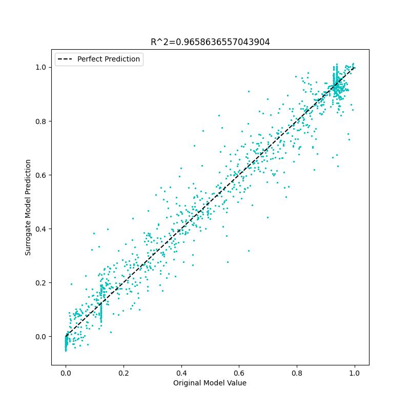
As it turns out, difficulties in modeling neural networks after mechanistic models is well-known within the scientific machine learning community (link here for a review of related work). One such well-documented difficulty is in modeling unbounded systems where parameters and their corresponding model outputs differ across various orders of magnitude, which is often missing in conventional supervised learning tasks. Applying this surrogate deep learning approach to two stochastic (i.e gillespie) nonlinear models, one a spatial agent based model and the other a non-spatial nonlinear 6 protein reaction network, naively applying a neural network without any feature transformations (i.e standardization, min-max scaling, etc.) leads to very some remarkably poor results. Here are some early results of what the surrogate fits looked like for the two nonlinear models.
Schematics for Both Nonlinear Models.

Nonlinear 6 Protein Reaction Network Surrogate Fit
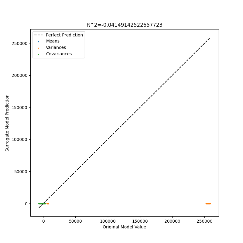
Spatial ABM (Giuseppe's Model Fit)
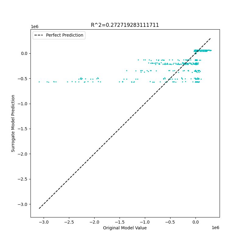
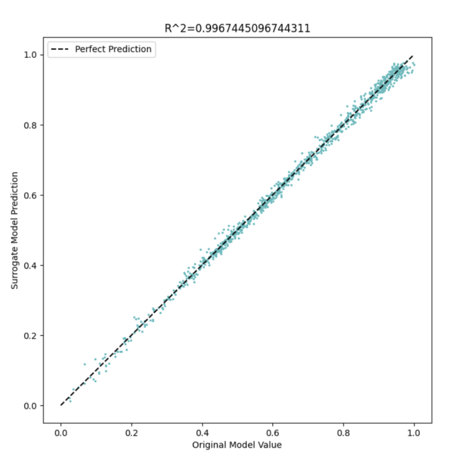
A way to mitigate these issues is to simply perform min-max scaling (or standardization) on the output feature vectors such that the feature space across all parts of the vector are bounded near 0. In the same order, we have the following improved fits
However, as one can see in the scatter plots, this still doesn't truly fully resolve all difficulties of fitting. There is still quite a bit of error surrounding the perfect fit line. While I haven't yet validated the nonlinear 6 protein reaction network's predictions with the actual model (as its fit isn't too bad), looking at the spatial ABM's fit, and one can reasonably assume it would have large approximation errors of the actual model and therefore be unsuitable for predictive purposes (and parameter estimation).
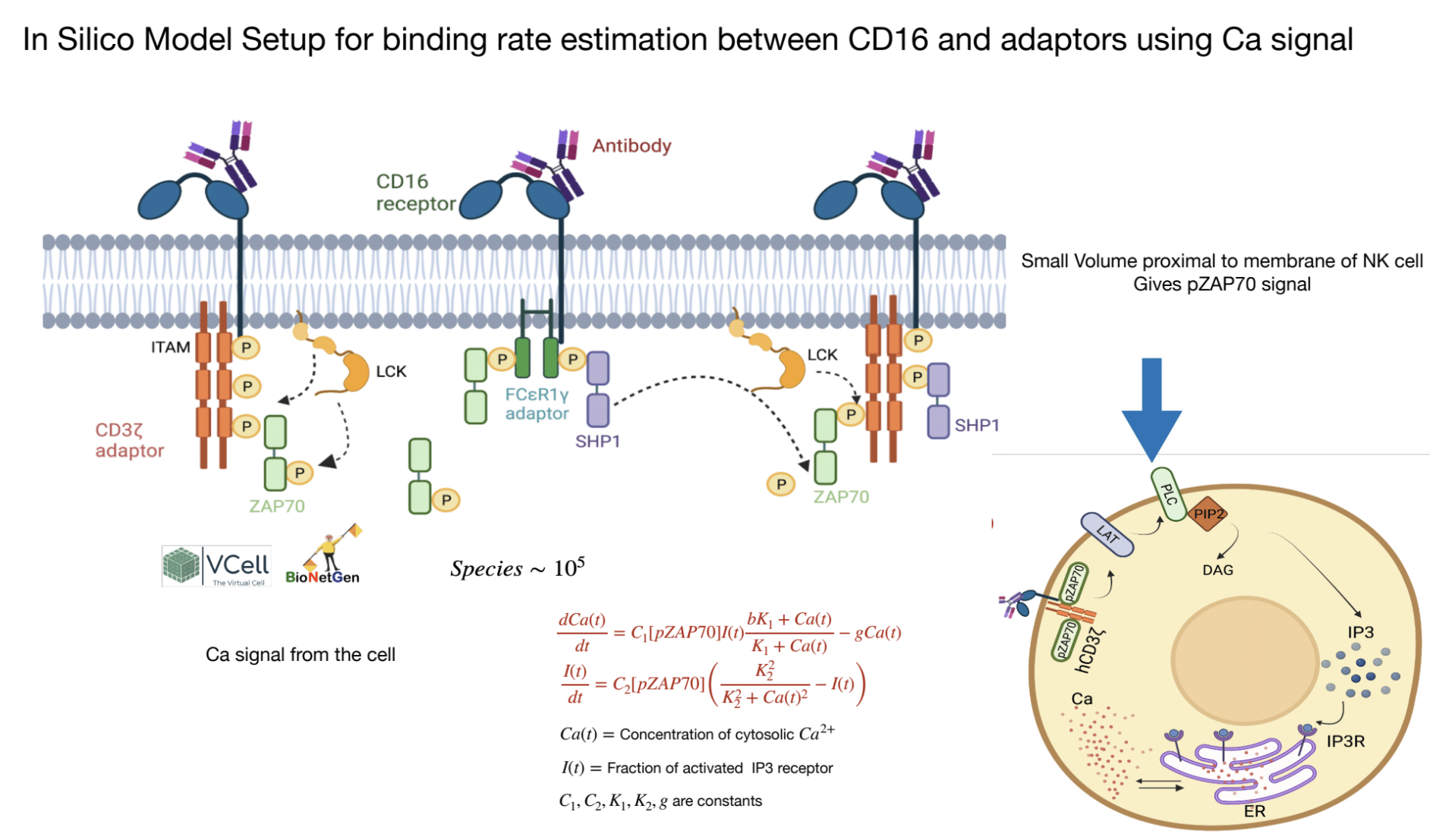
Furthermore, this type of error is further explored with Indrani's NFSim model below. (Apologies Indrani, I'm still too uneducated to understand what is going on with all of these crazy binding reactions.)
Here are some "decent fits". Note that I'm only showing one fit here at one time slice for one surrogate model (since the majority of the fits of these time slices are fairly similar). This was actually an attempt at doing parameter estimation with 4 surrogate models at 4 different time points, which is what is evaluated in the validation plot below.
But, when validated against the true model using previous estimates that are supposed to fit some curve, we get horrible results. Note that each color corresponds to a unique parameter set.
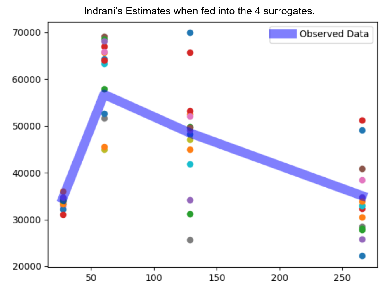
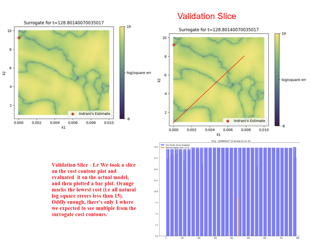
Furthermore, when looking at the cost spaces (confined by the training set's parameter bounds) with some observed data, you get some very wacky results. Comparing it to the true cost space (red line, we only evaluated a diagonal slice on the mechanistic model to save computational time as it's very expensive), we get the following plots.
(Note that lighter colors in the contour plot indicate higher cost.)
Dumb Possible Thoughts Why It's Hard to Take This Conventional Approach onto Indrani's Mechanistic Model
- Unbounded parameter space where parameters vary across many orders of magnitude (i.e C1 ~ 10^3 vs. k1 ~ 10^-7)
- Multiple Combinations of Parameters That Have the Exact Same Outputs (Maybe The Result of Unobserved Information from a Massive Model That has 1000's of RXNs)
- Irregular Cost Space (one needs to actually run the simulations to check, maybe highly sensitive? requiring more data)
- Since it's unbounded, possibly the training set doesn't contain a set of parameters that fit the observed data (initial experiments show that if you zoom in and create a training set of parameters around a set of parameters that fit the observed data with the actual mechanistic model, the surrogate can work on the inverse problem and return a set of valid parameters)
- Some future directions might be to build a larger training set around one of the estimates, and see if one can in principle get a valid surrogate model.
- Furthermore, there's a lot of information across time that isn't being used in these surrogate models, which may improve parameter estimation with surrogate models.
The arguably simplest method of building a direct mapping of parameters to some mechanistic outputs may not fully encompass the complex stochastic behaviors of certain models, especially when one considers biochemical reactions to be of time-series rather than simply just a snapshot in time and many models to have a spatial component. Such is the case with the spatial ABM depicted above. Unfortunately, I never had the time to truly explore all of the different conventional machine learning models (nor the time to use regularization methods such as dropout, L2 loss with the weights being a regularizer, etc.), here's a quick and dirty list of my naive attempts at using different neural network architectures for different mechanistic models and some statements on some things that I've noticed but never had the time to make graphical plots for.
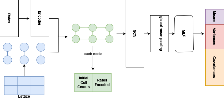
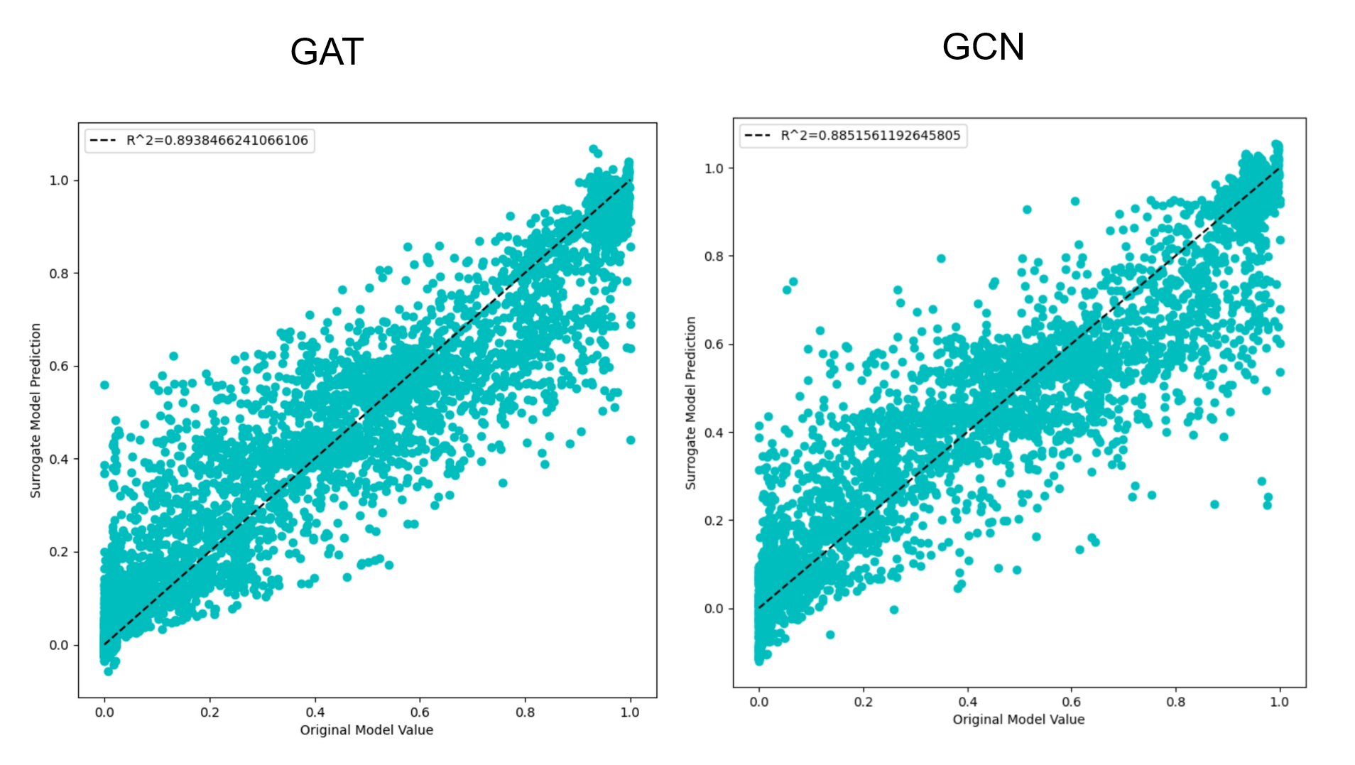
Exploring graph convolutional neural networks and graph attention networks used to act as a surrogate model for Giuseppe's model has shown that naive guesses are often just that, naive guesses. In particular, in a spatial ABM (or gillespie), a specific pixel (or position on a grid) has a variety of ways to update based on its neighboring pixels, and therefore in a way, it acts like a node on a graph. As such, one can (naively) imagine, that using graph neural networks where nodes are updated through some forwarding method and also nonlinearly transformed by some sets of weights (and their corresponding nonlinear activation functions), would do a reasonable job in acting as a surrogate for a spatial agent based model. The following architecture attempted with the surrogate model and their corresponding fits are shown below.
Architecture for GCN and GAT (note that the GCN unit is interchangeable with the GAT).
Their corresponding GCN and GAT fits respectively.
 Here's what it looks like when you color code them by their moment type.
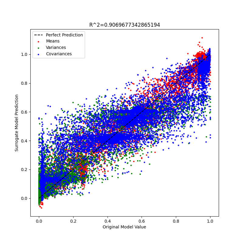
While this may seem like a slight improvement over the original multilayer perceptron surrogate model (and actually a lower R^2 value), there's potentially even more gains to be had. Here are the following things that I've never gotten to explore, but wish that I had the time for:
- Generate More Data
- Generate a dataset with outputs based on an earlier time point. (This simulation was simulating interactions between immune cells and cancer cells for a duration of two weeks). Less time points might mean less intrinsic noise within the dataset and less dramatic changes across the grid.
- Try different types of graphs (i.e different definitions of nodes and edges). I had designed a massive graph where every pixel out of the (100 x 100) grid was a node and its nearest neighbors had edges connected to it. Such a graph might be too big and honestly naively might have many empty or insufficient edges that are useless in the final prediction. Other issues include the scale of the time where cancer can often traverse multiple pixels, meaning there might be a need for a global set of edges.
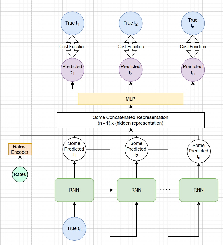
At some point, it felt worthwhile exploring time-series prediction models to maybe better incorporate temporal information within its parameter to output mapping. However, increasing the complexity of the datasets ran into complications as you'll soon see. Below we have the schematic of the surrogate model (and note the modules/model/temporal should contain the actual surrogate models). Furthermore, this input length determines how accurate
There's a trade-off between accuracy and the amount of observed time points you define as part of your input to the surrogate. While the figure above only shows one initial observed time point of your sequence, in principle, the sequence length that one feeds into the RNN or LSTM is variable. This can have varying effects on performance, especially should one naively choose to train the LSTM to predict only one time point into the future (where the input sequence is the entire trajectory missing the last time point and the output sequence missing the first time point).
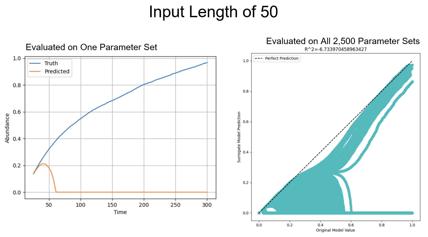
Here is an example of fits evaluating on an input sequence length of 50.
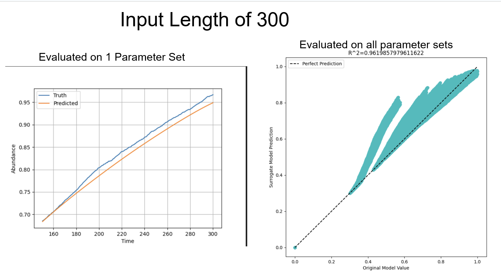
Here is an example of better fits evaluating on an input sequence length of 300. Note that a sequence of length 300 is only half the time points (i.e time 150 not the 300 on the plot shown).
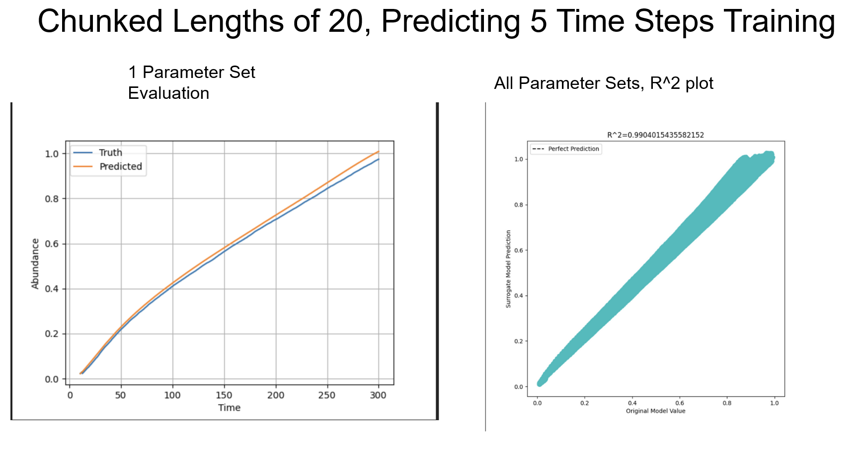
This leads to the next question of how one should train LSTMs to better predict the future time points, which brings into the question of chunking where instead of feeding the LSTM entire sequences, we feed it chunks of that sequence. Here we see a fit using a chunk size of 20 and attempting to predict 5 time points into the future, which dramatically improves the time-series predictions.
Transformer Models (Indrani's Network Free pZap and Ca Model) (With a Possible Application to Giuseppe's Model)
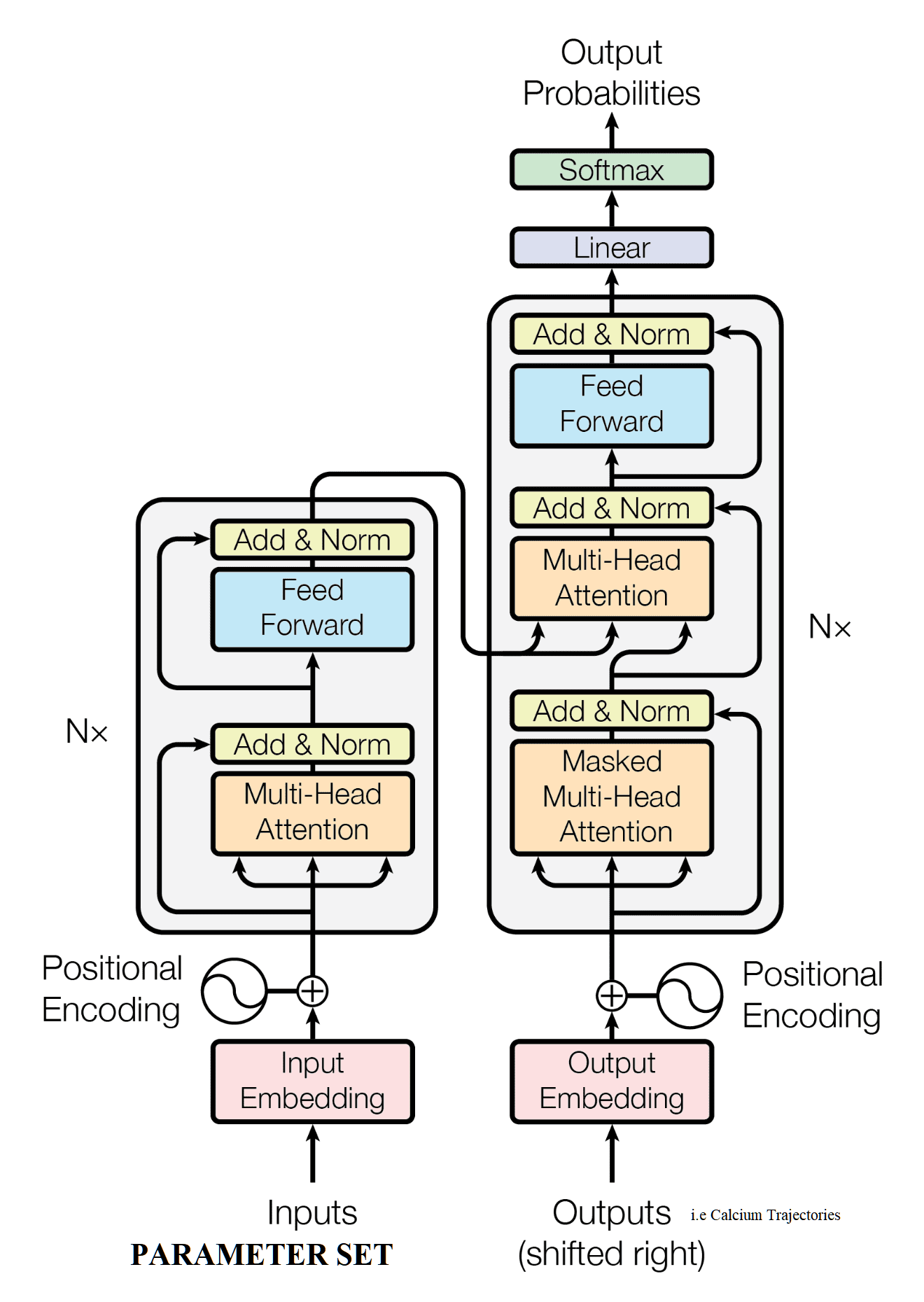
However, this type of fit in time-series predictions can be deceiving, as our goal isn't to predict the so-called observed future of the original mechanistic model given some input sequence, but rather the prediction of a trajectory given a set of changeable parameters. A good analogy is skydiving, a newbie skydiver can probably easily predict where he's falling to, but it's a different story if one wants to actually fly in the direction he's decided. Jumping into transformer models (taking inspiration from the NLP community), one might expect to see something like the following fits across all parameter sets in the test set. Furthermore, the dataset evaluated contains multiple features (pZap, Ca, h) changing across time rather than just the one (pZap) we've been exploring above with LSTMs. Below, we have some diagram of a transformer model and their inputs / outputs that I've taken and modified from google images to quickly showcase the off-the-shelf architecture, and then its corresponding fits to time-series data on an R^2 plot.
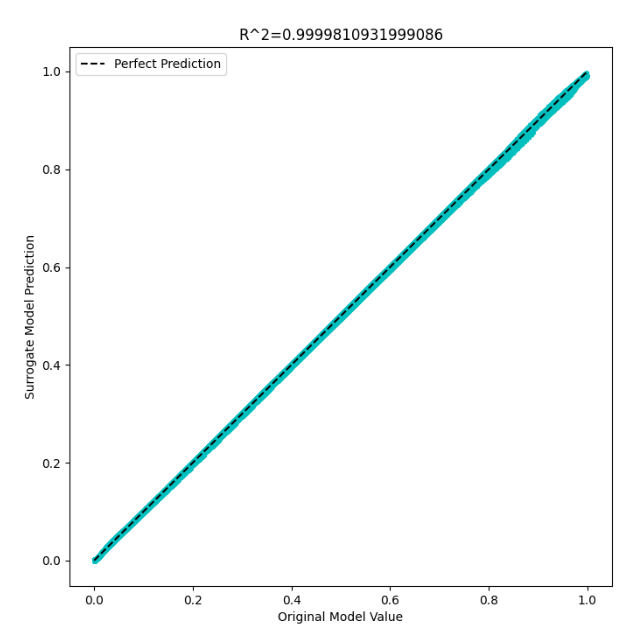
Here's the original starting attempt in just predicting one time point into the future, which unsurprisingly gives you a perfect fit in the R^2 plot.
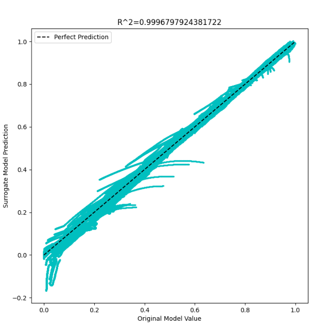
Here's the R^2 plot when attempting to predict 800 time points into the future, which is still surprisingly pretty good considering how little information it has from the original sequence.
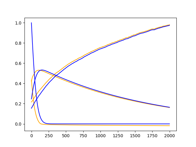
However, as earlier discussed, these plots are deceiving, especially when one considers the utility of these surrogate models is to map interpretable mechanistic model parameters to mechanistic model outputs and not just black box predictions. As such, suppose I fed in a set of 0 parameters (i.e no reactions, nothing is happened in the mechanistic model) to the transformer surrogate model that should in principle predict "0" or flat trajectories as nothing is supposed to be happening. Inputting this zero parameter set with some input sequence, we get surrogate predicted trajectories (orange) that perfectly fit trajectories that have non-zero parameter sets (blue).
In other words, the parameter set inputs to the transformer surrogate model had zero effect on the time-series prediction, meaning it had learned to predict future sequences only from the input sequence. This is something of a phenomenon in deep learning called shortcut learning.
Please look at requirements.txt for all of the used Python libraries. To install, simply do
pip install -r requirements.txt
To those in the Das lab that might be taking up the flag in developing this project further, for a quickstart, one can simply look in the /tutorials/tutorial_for_indrani.pynb notebook for a quick rundown on how one might use the pieces of code written. There's also a cli interface that I've provided with main.py, please look in the slurm_scripts/ folder for a plethora of shell scripts used to run the code on the cluster. The flow chart below provides a general workflow of the surrogate modeling done in this repository (cross validation in principle should be used, but there's a tradeoff in computational time vs. generalization error to be had when using cross validation).
Please look in the modules/ folder for relevant pieces of code.
Other potential future directions (that I wish I had the time for), taking inspiration from the general machine learning communities.
Dr. Das, I think someone should pursue the idea of treating sequences as shapes (like a triangle) rather than anything else really interesting. I wish I could've properly pursued this idea further.
- Dr. Stewart brought up the idea of using hundreds of surrogate models since smaller models can be in principle faster to train, and much faster to evaluate than the original model. Funnily enough, someone's attempted this with partial differential equations here (even if our problem is different because we are tackling stochastic models rather than deterministic).
Papers from related fields that attempt to do something similar to what we're doing, but I haven't had the time to read thoroughly and truly understand the major ideas (and why they might work and not work for our case).
- Synthetic Data Generation for Molecular Time-Series Data
- Using CNNs for Surrogate Modeling for Connectivity Prediction for Work Layouts
- GNN Surrogates for Unstructured Ocean Simulations <- Understanding this might be key to improving our spatial surrogate models.
- Review of Surrogate Models and Their Application to Groundwater Modeling
- A review on design of experiments and surrogate models in aircraft real-time and many-query aerodynamic analyses
Since it is now the era of fine-tuning and "pre-training" in the NLP and vision fields, it's interesting that it hasn't heavily spread into the domain of scientific machine learning. There could be various reasons for this, but ultimately, if one could in principle take a pre-trained surrogate model and fine-tune it to properly surrogate another related mechanistic model, one could in principle speed up training by 100x. If we could get a useful surrogate model off the ground, this would be a solid research direction. It's interesting to note that people are already attempting to do this for deterministic mechanistic models as seen with the physics-inspired neural networks community.
I've tried this with no luck in actually getting some of their packages to run, and I figured at the time, it wasn't worth further exploring. But, if you can simply blackbox the training approach, and it works, I don't see why not giving it a shot.
Thank you Dr. Stewart, Dr. Jay, and Dr. Das for basically acting as 3 senior research mentors to essentially just an undergrad. I recognize how lucky I am to have been able to take up the valuable time. I think it's funny that I didn't realize until I had Darren point it out to me, that I basically had the firepower of 3 PI's giving me advice on my one project. I think I would've been much more lost had I not had this level of support that has shaped my thinking in this amazing world of open research.
Thank you Darren and Giuseppe, the awesome PhD students within the lab, for giving me advice, shaping my belief and desire to do a PhD, and honestly just providing company on the days I came into the office. It's often nice to have people who are willing to listen your research woes and talk about stuff outside of research.
Thank you Mahesh for being my walk-home buddy as well as also providing valuable advice and insights in aiding with my research. I hope you figure out the nuances of neural turing machines. Funnily enough, I read somewhere, they might be part of the next steps towards general ai.
Thank you Indrani, Debanghana, and everyone else in the Das lab (that I might've forgotten about) for helping me understand their research and taking the time to explain it to a dummy like me.
