sumo_carla_simulator

Introduction of the Project

About

This project contains the source code and data for "xxxx".

Features

Users can use this repo to generate testing trajectories, process and analyse simulation results.

Code Structure

'main.py' runs vehicle testing simulations and generats raw trajectory data, which depends on 'envs', 'conf', 'controller', 'maps', 'source_data' and 'mtlsp'. 'envs' specifies NDE and NADE driving environments which utilizes vehicle controllers from 'controller' and maneuver probabilities from 'source_data'. 'mtlsp' combines 'envs' and 'maps' and runs SUMO simulations. 'data_analysis' folder contains two folders: 'processed_data' and 'analysis_and_figures'. 'processed_data' contains notebooks that process raw testing data into metrics including crash rate, crash type severity, near miss TTC and PET. 'analysis_and_figures' provides notebooks to analyse the metrics and plot their distributions.

An illustration is as follows:

D2RL/
- conf: configurations for raw data generation and data analysis
- maps: maps for data generation
- checkpoints: model checkpoints for D2RL in raw data generation step
- source_data: source data to estimate vehicle maneuver probabilities in raw data generation
- mtlsp: the mtlsp repo uses SUMO to simulate driving in given environment with given controllers
- envs: environments for mtlsp to run simulations in
- controller: vehicle controllers for mtlsp environments
- data_analysis: the main folder for data analysis
  - raw_data: either self generate or download from our G-drive, the raw vehicle trajectories from SUMO simulation
  - processed_data: notebooks to process the raw data into performance metrics including crash rate, crash type severity, near miss TTC and PET.
  - analysis_and_figures: notebooks to analyse the metrics and plot their distributions.
- main.py: run simulation with mtlsp and generate raw data
- utils.py: utility functions
- nadeinfoextractor.py: information extractors that document information at each timestep of the experiment
- requirements.txt: required packages for this repo to run

Installation

Pre-requirements

Python installation This repository is developed and tested under python 3.10.4 on Ubuntu 20.04 system.
Download all required datasets Due to the size limit of the github, the raw data and some processed data cannot be uploaded. Therefore, we store the data_analysis folder in the Google Drive. The user should download the data_analysis folder from here. Then, the user should merge the downloaded data_analysis folder with the original data_analysis folder in the repo.

Installation and configuration

Clone this repository

git clone https://github.com/michigan-traffic-lab/Dense-Deep-Reinforcement-Learning.git

Create a new virtual environment (Optional)

A virtual environment is recommended to be utilized to run this repo, as it can provide high flexibility. To install the virtual environment, please use the following commands:

virtualenv venv
source venv/bin/activate

Install all required packages

This repository is built based on several python packages, which can be installed using the following command:

pip install -r requirements.txt

Post-installation steps

Before running jupyter notebooks in the data analysis, the ipykernel is needed. To install it, users can run the following command:

pip install ipykernel

Usage

All the data, code, and results are stored in /data_analysis folder. In this project, several performance metrics are analyzed, including time-to-collision, post-encroachment-time, bumper-to-bumper distance, crash rate, crash type, and crash severity. In this section, we will use the post-encroachment-time (PET) analysis as an example, while all other performance metrics follow the same procedure. The code for each performance metric analysis is stored in a separate jupyter notebook.

For jupyter notebook usage, please refer to https://docs.jupyter.org/en/latest/

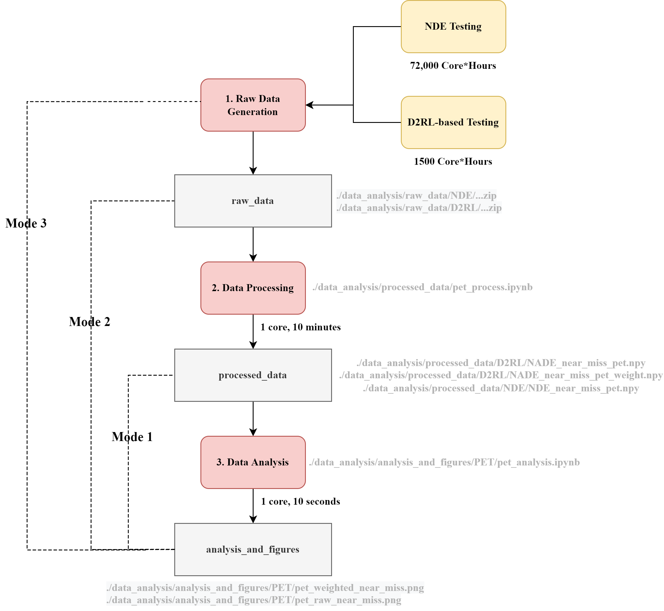
For the convenience of usage, we provide three running modes as illustrated in the following figure. Specifically, there exist three steps to reproduce the experiment results:

1. Raw data generation
2. Data processing
3. Data analysis

As the raw data generation is time-consuming (e.g., 72,000 core*hours are needed for the NDE testing experiment), we also provide the data generated in our experiments, so users can use the data to skip the first two steps (Mode 1) or the first step (Mode 2) for quick reproduction. Specifically, there are three running modes as follows:

Mode 1 (recommended): data analysis (step 3) using the data generated in our experiments;
Mode 2: data processing (step 2) and data analysis (step 3) using the data generated in our experiments;
Mode 3: raw data generation (step 1), data processing (step 2), and data analysis (step 3).

1 core*hour denotes the simulation running on one CPU core (Intel Xeon Gold 6154 3.0GHz) for one hour.

To provide further details of the three code running modes, a flowchart of PET data generation, processing, and analysis is provided as follows:

1. Raw Data Generation

For Mode 1: this step is skipped.
For Mode 2: this step is skipped
For Mode 3:
- Please run the following commands to run the simulation and generate the raw experiment results for Naturalistic Driving Environment (NDE) testing and D2RL-based testing (the experiment_name can be specified by users):
  - ```
  python main.py --experiment_name 2lane_400m_NDE_testing --mode NDE # Use this for NDE Testing
```
- ```
python main.py --experiment_name 2lane_400m_D2RL_testing --mode D2RL # Use this for D2RL Testing
```
  - By default, the simulation result will be stored in ./data_analysis/raw_data/experiment_name.

2. Data Processing

For Mode 1: this step is skipped.
For Mode 2:
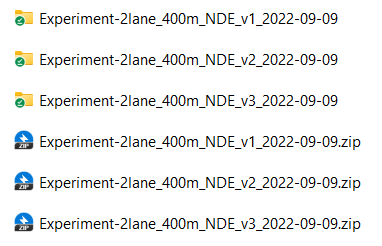
- Before running mode 2, the dataset under /data_analysis/raw_data needs to be unzipped first. All zipped files should be unzipped to the same directory. Please note that the unzip process could take about 30 minutes and the total size of the unzipped files is around 130 GB.
  - For D2RL experiment results, the zipped file and unzipped folders should follow the file structure as shown in the following figure:
  - For NDE experiment results, the zipped file and unzipped folders should follow the file structure as shown in the following figure:
- Run all the code cells in the jupyter notebook (click "Run all" button in the menu bar of the notebook)
- The processing code is stored in /data_analysis/processed_data/. For example, the processing code of the PET for both NDE experiments and D2RL experiments can be found in the jupyter notebook pet_process.ipynb, including several major procedures:
  - Load raw experiment results
  - Data processing: transfer raw information (e.g., speed and position) to performance metrics (e.g., PET)
  - Store the processed data into /data_analysis/processed_data/NDE or /data_analysis/processed_data/D2RL
  - After the data processing, you should be able to find newly generated files:
    - NADE_near_miss_pet_weight.npy and NADE_near_miss_pet.npy under /data_analysis/processed_data/D2RL
    - NDE_near_miss_pet.npy under /data_analysis/processed_data/NDE

For Mode 3:

Please modify the following codes in the jupyter notebook to process the newly generated experiment results:

root_folder = "../raw_simulation_results/D2RL/" # Please change it to the position where you stored the newly generated raw experiment data
path_list = ["Experiment-2lane_400m_IDM_NADE_2022-09-01"] # Please change it as the name of the folder generated in your new experiments

After the modification, users can follow the data processing for Mode 2.

3. Data Analysis

This step is the same for all three running modes.

All the data analysis codes and generated figures can be found in /data_analysis/analysis_and_figures/. The file structure is as shown in follows:

data_analysis/
|__ raw_data
|__ processed_data
|___analysis_and_figures
|______ crash_analysis
|_________ crash_severity_type_plot.ipynb # Analyze the crash severity and the crash type
|______ crash_rate
|_________ crash_rate_bootstrap_plot.ipynb # Analyze the crash rate, the convergency number
|______ near_miss_TTC_distance
|_________ ttc_distance_analysis_json.ipynb # Analyze the TTC, bumper-to-bumper distance
|______ PET
|_________ pet_analysis.ipynb # Analyze the PET

For example, the PET data analysis code can be found in /data_analysis/analysis_and_figures/PET/pet_analysis.ipynb, including the following major procedures:

Load the processed experiment data from /data_analysis/processed_data
Plot the PET histogram of D2RL experiments and NDE experiments, and then save the figures to /data_analysis/analysis_and_figures/PET.

Contributing

Contributions are what make the open source community such an amazing place to be learn, inspire, and create. Any contributions you make are greatly appreciated.

Fork the Project
Create your Feature Branch (git checkout -b feature/AmazingFeature)
Commit your Changes (git commit -m 'Add some AmazingFeature')
Push to the Branch (git push origin feature/AmazingFeature)
Open a Pull Request

License

H. L. and the team have filed a US provisional patent application 63/338,424.

Developers

Haowei Sun (haoweis@umich.edu)

Haojie Zhu (zhuhj@umich.edu)

Shuo Feng (fshuo@umich.edu)

For help or issues using the code, please create an issue for this repository or contact Haowei Sun (haoweis@umich.edu).

Contact

For general questions about the paper, please contact Henry Liu (henryliu@umich.edu).

jingxuanyang/sumo_carla_simulator