Machine Learning Approach for Bridging Solution X-ray Scattering Data and Molecular Dynamic Simulations on RNA
This ML approach was published in IUCrJ:
Please refer to WAXS-XGBoost-Radius-Training.ipynb in this repo for the notebook mentioned in our manuscript. If Github has trouble parsing the notebook, try either download it or view the WAXS-XGBoost-Radius-Training.pdf.
- xgboost (version: 0.9.0)
- numpy (version: 1.16.4)
- scikit-learn
- pickle
- h5py (version: 2.9.0)
- Testing the linear models (linear regression, ridge regression and LASSO):
linear_radius.py - Exploring the Shannon sampling limit and noise effects:
xgb_radius_sampling_noise.py
- If you find it useful, please cite the paper. Thanks.
- The following is just "garbage collection".
- I also tried 1D convolutional neural network (CNN), which also worked but not as simple and interpretable as the xgboost models. The CNN approach was presented at Biophysical Society Meeting 2020 in San Diego and you can find the abstract here.
- The CNN models were implemented in (a) Python using
keraswithtensorflowbackend and (b) Julia usingMocha.jl, which has migrated toMXNet.jlorFlux.jl.
Convolutional Neural Network (CNN) Approach for Solution X-ray Scattering Data
Convolutional Neural Networks Bridge Molecular Models and Solution X-ray Scattering Experiments
- keras with Tensorflow backend (version: 2.2.4)
- pickle
- numpy (version: 1.16.4)
- h5py (version: 2.9.0)
- Setting up the function
convolutional_neural_netsandtrain_modelby running
runfile('/my/path/to/training.py', wdir='/my/path/to')And keras should tell you:
Using TensorFlow Backend
- Setting up the convolutional neural network by running
model = convolutional_neural_nets()One should see the structure of the network as the following.
_________________________________________________________________
Layer (type)                 Output Shape              Param #
=================================================================
conv1d_1 (Conv1D)            (None, 191, 128)          1408
_________________________________________________________________
activation_1 (Activation)    (None, 191, 128)          0
_________________________________________________________________
dropout_1 (Dropout)          (None, 191, 128)          0
_________________________________________________________________
max_pooling1d_1 (MaxPooling1 (None, 92, 128)           0
_________________________________________________________________
conv1d_2 (Conv1D)            (None, 92, 128)           163968
_________________________________________________________________
dropout_2 (Dropout)          (None, 92, 128)           0
_________________________________________________________________
max_pooling1d_2 (MaxPooling1 (None, 43, 128)           0
_________________________________________________________________
conv1d_3 (Conv1D)            (None, 43, 128)           163968
_________________________________________________________________
dropout_3 (Dropout)          (None, 43, 128)           0
_________________________________________________________________
max_pooling1d_3 (MaxPooling1 (None, 18, 128)           0
_________________________________________________________________
flatten_1 (Flatten)          (None, 2304)              0
_________________________________________________________________
dense_1 (Dense)              (None, 1024)              2360320
_________________________________________________________________
batch_normalization_1 (Batch (None, 1024)              4096
_________________________________________________________________
dense_2 (Dense)              (None, 256)               262400
_________________________________________________________________
dropout_4 (Dropout)          (None, 256)               0
_________________________________________________________________
dense_3 (Dense)              (None, 64)                16448
_________________________________________________________________
dropout_5 (Dropout)          (None, 64)                0
_________________________________________________________________
dense_4 (Dense)              (None, 25)                1625
=================================================================
Total params: 2,974,233
Trainable params: 2,972,185
Non-trainable params: 2,048
_________________________________________________________________
Alternatively, you can print this out by typing:
model.summary()One can change the indim, outdim, n_filters, conv_kernel, conv_stride, pool_kernel and pool_stride to try it out for your problem of interest.
- Training
Use the function train_model and input the training data. See the file training_script.py for details.
Once the training begins, the interface looks like the following:
...
43235/43235 [==============================] - 0s 63ms/step - loss: 0.4817 - acc: 0.7708
Epoch 147/2500
43235/43235 [==============================] - 0s 64ms/step - loss: 0.4764 - acc: 0.7747
Epoch 148/2500
...
The hyper-parameters at the training stage are: learning_rate, batch_size and n_epochs but are not restricted to these. The hyper-parameter tuning is difficult for some problems.
The trained model will be saved as *_model_yyyymmdd.h5 file for further analysis and testing.
- Load model
To load your trained model, run
from keras.models import load_model
model = load_model("*_model_yyyymmdd.h5")These plots were in my BPS2020 poster.
- CNN structure
- Training History and Performances
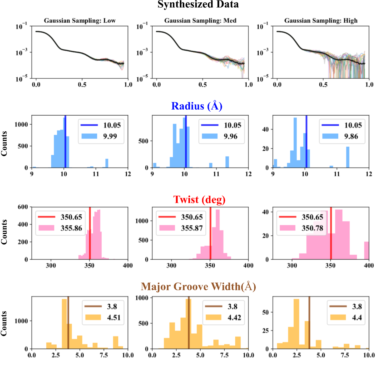
- Validation on Sythesized data
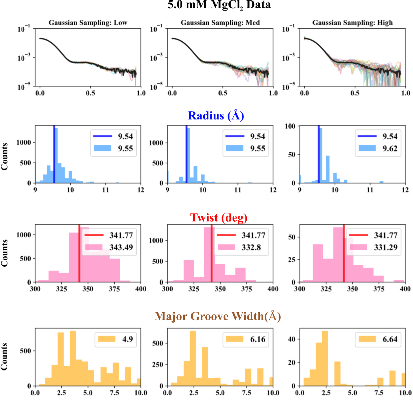
- On experimental data
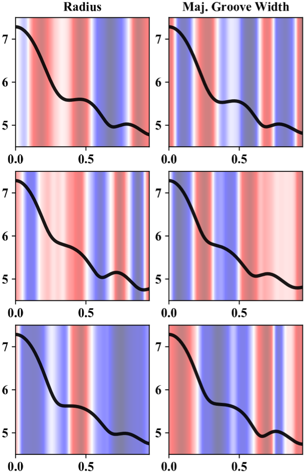
- First CNN layer output (feature importance/information)
- Please check out the documentation of keras for more detailed information
- The structure of neural network might depend on different problems
- The following is another "garbage collection".
Generalized Convolutional Neural Net for Solution X-ray Scattering Data
- I was being too, over, ambitious.
- I didn't have enough computing resources at Cornell, but the data prep is done ~ 2T.
- There is a nice work that "sort of" shares the same idea: Model Reconstruction from Small-Angle X-Ray Scattering Data Using Deep Learning Methods
Mocha.jl(nowMXNet.jlorFlux.jl)CLArray.jl(nowCuArray.jlorGPUArray.jl)Dierckx.jl
- The file
networks.jlcontains the CNN models and the feed-forward models. - The file
dq.jlhas been integrated to my other packages:SWAXS.jl(private) andSWAXS(binary). - Special thanks to Princeton CS group


