2110446-DS-and-DE

code in DS and DE class

2110446-DS-and-DE

Acknowledgement

the folder example_code and example_slide is from the class github(referred in Reference)
all assignment is from the class github(referred in Reference)

1st week

key pandas command

# pandas command

## from 3rd python notebook
map(...)
apply(...)
cut(...)
unique(...)
filter(...)
### key datetme transformation

## from 4th python notebook
file.json(...)
df.merge(...)

Assignment 1

link here

2nd week

interest command

import pandas as pd
df = pd.read_csv(...)

# drop row/column
df.dropna(tresh=x) # drop which value not fit treashold
df.drop(columns=[...])

'''
axis 0=row, 1=column
'''

# count by values
df[...].value_counts()

# count Null/None value
df.isnull().sum()

# mapping dict
md = {
    col_name1 : {
        from1 : to1,
        from2 : to2,
        ...
    }
    col_name2 : {...}
}
df.replace(md, inplace=True)

# One-hot encoding
dummied_df = pd.get_dummies(df[col_name], drop_first=...)
#   or use scikit-learn (better)
from sklearn.preprocessing import OneHotEncoder
oh_enc = OneHotEncoder(drop='first')
oh_enc.fit(X)
#   can use with both train and test but use parameter that fitted

# impute missing
from sklearn.impute import SimpleImputer
num_imp = SimpleImputer(missing_value=..., strategy='mean')
num_imp.fit(X)
#   can use with both train and test but use parameter that fitted

# train/test split
#   note that y must be category so if y is numeric -> add grouping column
from sklearn.model_selection import train_test_split
X_train, X_test, y_train, y_test = train_test_split(X,
                                                    y,
                                                    stratify=y,
                                                    test_size=...,
                                                    random_state=42)

# remove outlier
from scipy import stats
#   1. mean +- 3sd (z>3 or z<-3)
z = np.abs(stats.zscore(df))

Week 3

AI

has

Rule-based AI
- Knowledge representation
- create Answer from data and rule
Machine learning
- create Rule from data and answer
- scikit-learn for traditional

Supervise learning (Predictive task)

learn from existed answer

the methodology

Training phase
- give data to model
Testing phase (inference)
- evaluate perfomance
- use model in real problem

Type of problem

Classification problem
- target is categorical problem
- use classifier model
Regression problem
- target is predict numeric
- use regressor model

Unsupervise learning

learn from only data (no answer)

Impurity reduction

Entropy
Information Gain
- $\text{Information Gain} = Entropy_{Before} - Entropy_{After}$
Gini impurity
- $Gini = 1-\sum_{i}^{n}(P_i)^2$
  - $P_i$ : prob. of class i in data-set
- $\text{Gini reduction} = Gini_{Before} - Gini_{After}$

Tree visualization

from sklearn.tree import plot_tree

plot_tree(model)

Regularization

balance between performance and complexity

Dicision tree classifier

make decision based on node criteria
each leaf node represents area and % of confidense is from ratio between class

essentials

split search - compare impurity between before and after split and select best purity from the split
after get splitted area -> recursive on each area.

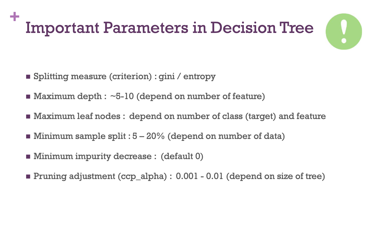
hyperparameters

max_depth : maximum depth of the model
- the more max_dept, the more overfitting
min_leaf_size : minimum datapoints in each leaf(area)
- the less min_leaf_size, the more overfitting

Adventage

the model is decribable
able to tell feature importance
- summation of $\nabla\text{goodness}$
- use for variable selection
- model.feature_importances_

Be caution

Instability
- very sentitive to datapoints. model change with a little noise

Pruning

$ R_\alpha (T) = R(T) + \alpha|T|$
use $\alpha$ to regularization the three
the more $\alpha$, the smaller tree
$\alpha$ is ccp_alphas in sklearn.tree but default is 0

Bagging ( Bootstrap Aggregation )

random with replacement

random subset
- each subset can be overlapping
use subset to train model ( get more model )
use each model to help predict together

Boosting

onvert waek learner to stronger one

in each step, we boost freq. the wrong case of the previous tree.
do any step until we accept the perfomance

e.g. AdaBoosting, XGBoost, etc.

Random forest classifier

random without replacement

random subset
- all subset must not overlapped both data and features
do like normal tree

hyperparameters

max_sample
max_featurea
n_estimators

hyperparameters

#Tree
#Columns (features)
#Rows (example)

Feature selection from tree (feature importance) with shortcut

from sklearn.feature_selection import SelectFromModel

model = ...
selector = SelectFromModel(model)
selector = select.fit(X, y)
selector.get_support()

Linear regression

assumption

linear relationship between feature and target
error are independent from each other
target distribution is normal (no outlier)
- error are normally distributed
- error have constant variance

Regularization

Idea : $\text{Loss} = \text{Error} + \lambda\text{Complexity}$
L1 : Lasso
- absolutely
- $ \text{Loss} = \sum_{i=1}^{n}(y_i - \hat{y_i})^2 + \lambda\sum_{j=1}^{p}|\beta_j|$
L2 : Ridge
- square
- $ \text{Loss} = \sum_{i=1}^{n}(y_i - \hat{y_i})^2 + \lambda\sum_{j=1}^{p}\beta_j^2$

Sklean example

from sklearn.linear_model import Lasso, Ridge, ElasticNet

model = Lasso(alpha=...)

model = Ridge(alpha=...)

model = ElasticNet(alpha=..., l1_ratio=...) # l1_ratio = 0 -> Ridge, l1_ratio = 1 -> Lasso

Basic solution

if not linear -> use Neural Network
if not normal -> take log to make it more normal

Week 4

kNNs

k : number of nearest neighbors -> to make vote/average/miximum prob, etc.
distance_fn : to measure distance

Caution

must be numeric value
must normalize data on each axis

GridSearchCV

from sklearn.model_selection import GridSearchCV
from sklearn.model_selection import StratifiedKFold

grid_search = GridSearchCV(estimator=...,
                           param_grid=...,
                           scoring=...,
                           cv=StratifiedKFold(n_splits=5))
grid_Ssarch.fit(...)

model = grid_search.best_estimator_

model.predict(...)

RandomizeSearchCV

as same as GridSearchCV but randomize approach
n_iter : to tell the most iteration to random select.

Save & Load model

import pickle

# to save model
pickle.dump(model, open('model.pkl', 'wb'))

# to load model
loaded_model = pickle.load(open('model.pkl', 'rb'))

loaded_model.predict(...)

Pipelining

from sklearn.impute import SimpleImputer
from sklearn.preprocessing import OneHotEncoder, MinMaxScaler
from sklearn.compose import ColumnTransformer, make_column_selector
from sklearn.pipeline import Pipeline

num_pl = Pipeline(steps=[('impute', SimpleImputer(strategy='mean')),
                         ('scale', StandardScaler())])

cat_pl = Pipeline(steps=[('imput', SimpleImputer(strategy='most_frequent')),
                         ('scale', OneHotEncoder())])

from sklearn.compose import ColumnTransformer

col_transf = ColumnTransformer(transformers=[('num_pl', num_pl, num_cols),
                                             ('cat_pl', cat_pl, cat_cols),
                                             n_jobs=-1], remainder='drop')

model_pl = Pipeline(steps=[('col_trans', col_trains),
                            'model', model])

# display pipeline
display(model_pl)

# to get parameters name
model_pl.get_params()

Neural Network

hidden_units, hidden_layers, lr, decay, etc.

from sklearn.neural_network import MLPClassifier, MLPRegressor

# solver is equal to Optimizer
'''
for example 2 layer that has 100, 200 nodes
si hidden_layer_sizes = (100, 200)
'''
model = MLPClassifier(hidden_layer_sizes=...,
                      actication='relu',
                      solver=...)

Weight updating

Stochastic Gradient Descent (SGD)
- update weight for every single iteration(each data point)
- note not tolerate to outlier
Batch Gradient Descent
- train all the data and average gradients to calculate back prop.
Mini-batch Gradient Descent
- group data into smaller batch and average bra bra bra
- note use less memory, tolerate to outlier.
- aka. batch_size

CNN

kernal
- filter size : size of kernel
- filters : number od kernel
- stride : number of pixel that kernel moved
- padding : number of pixel extended process convolution layer (feature extraction) -> NN -> outcomes

example

VGGNet
- feature extraction layer : Conv2D(3x3) + Conv2D(3x3) + MaxPool
Inception V1/ GoogLeNet
- variant kernel size
- Deeper and Wider
Inception V2, V3
- more speed
- Factorize metrix e.g. 5x5 kernal represented by 2 of 3x3 kernel, etc.
- use Batch norm to reduce Gradient vanishing
ResNet
- make Short skip connection then each group call residual block, to reduce Gradient vanishing
Inception-ResNet
- make Inception go deeper.
EfficientNet
- deeper, wider, resolution (variant size of kernel) -> compound scaling
EfficientNet V2
- smaller and faster 6x
- size : S, M, L, XL

Use case

Image classification (via CNN)

Setup

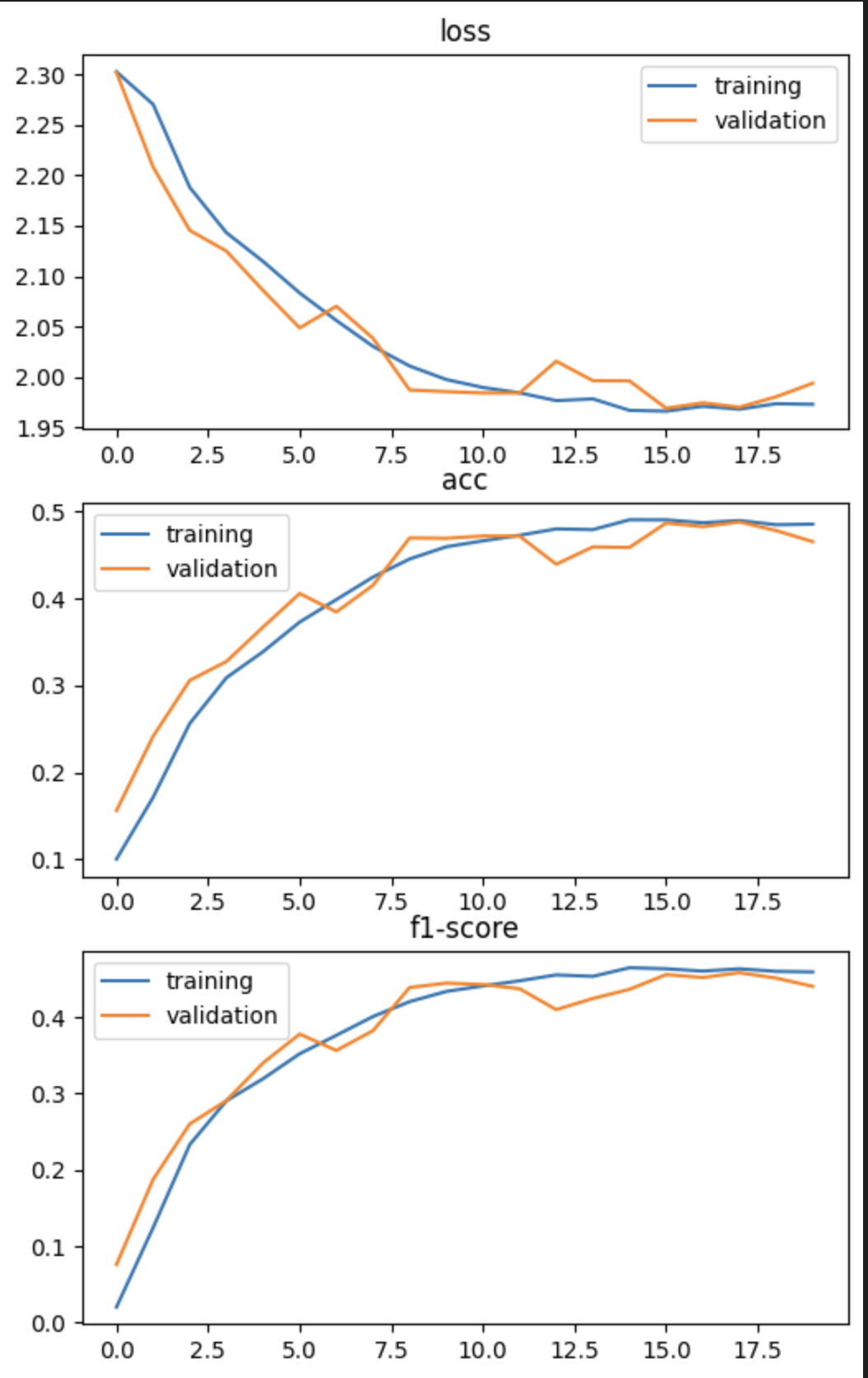
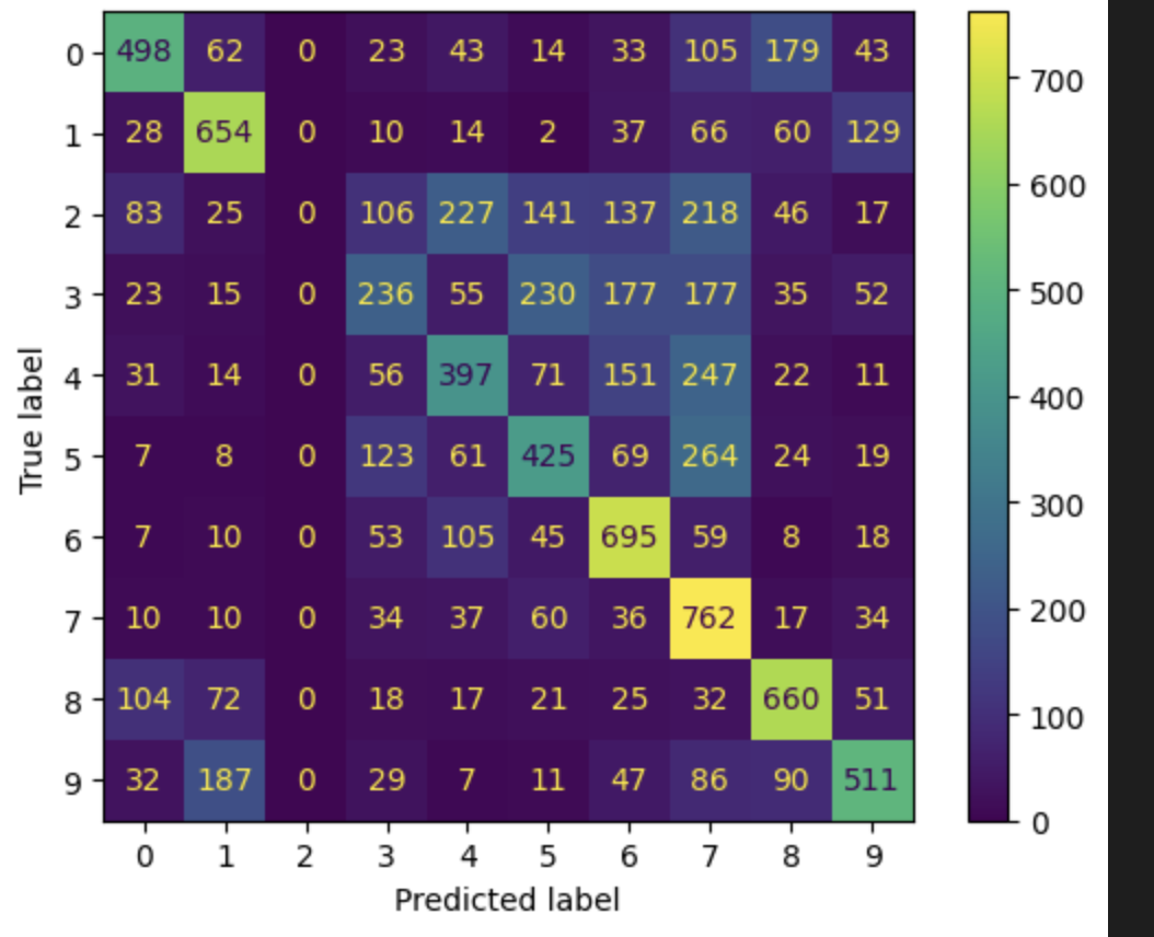
Classify image in CIFAR 10 dataset with CNN model
Use GPU for training
Input : image in size (32, 32, 3)
Output : 10 classes (0-9)
Batch size is 32
from 60,000 image splited into
1. 40,000 of train
2. 10,000 of validation
3. 10,000 of test

Model arch.

Conv2D (nn.Conv2d(3, 6, 5))
- input_channel = 3
- output_channel = 6
- kernel_size = (5, 5)
- parameters = (5x5)x3x6 + 6 = 456
ReLU (nn.ReLU())
MaxPool2D (nn.MaxPool2d(2, 2))
- kernal_size = (2, 2)
- stride = 2
Conv2D (nn.Conv2d(6, 16, 5))
- input_channel = 6
- output_channel = 16
- kernel_size = (5, 5)
- parameters = (5x5)x6x16 + 16 = 2,416
ReLU
MaxPool2D
- kernal_size = (2, 2)
- stride = 2
Flatten (torch.flatten())
Dense (nn.Linear(400, 120))
- input = 400 (16x5x5)
- output = 120
- parameters = 400x120 + 120 = 48,120
ReLU
Dense (nn.Linear(120, 84))
- input = 120
- output = 84
- parameters = 120x84 + 84 = 10,164
ReLU
Dense (nn.Linear(84, 10))
- input = 84
- output = 10
- parameters = 84x10 + 10 = 850
Softmax (nn.Softmax())

Total parameters = 456 + 2,416 + 48,120 + 10,164 + 850 = 61,006

from torchinfo import summary
print(summary(model, input_size=(32, 3, 32, 32)))

Training

Loss(criterion) : nn.CrossEntropyLoss()
Optimizer : torch.optim.SGD(model.parameters(), lr=1e-2, momentum=0.9)
train steps

Let's train! For an epoch in a range Call model dot train Do the forward pass Calculate the loss Optimizer zero grad Lossssss backward Optimizer step step step

Test time! Call model dot eval With torch inference mode Do the forward pass Calculate the loss

Print out what's happenin'

Let's do it again 'gain 'gain

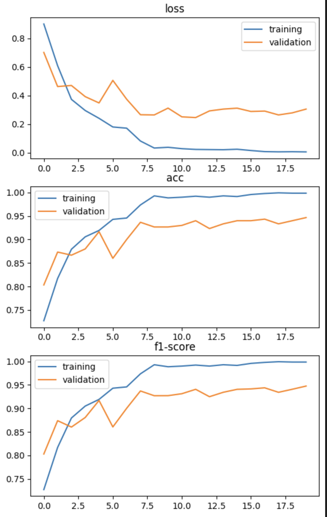
choose the model by validation loss

Training result

Metrics

report = classification_report(y_labels, y_pred)

acc = report['accuracy']
prec = report['weighted avg']['precision']
rec = report['weighted avg']['recall']
f1 = report['weighted avg']['f1-score']

Accuracy
- in prediction, how many correct
Precision
- in prediction, how many correct in positive
Recall
- in positive, how many correct in prediction
F1
- average of precision and recall

Evaluation (confusion matrix)

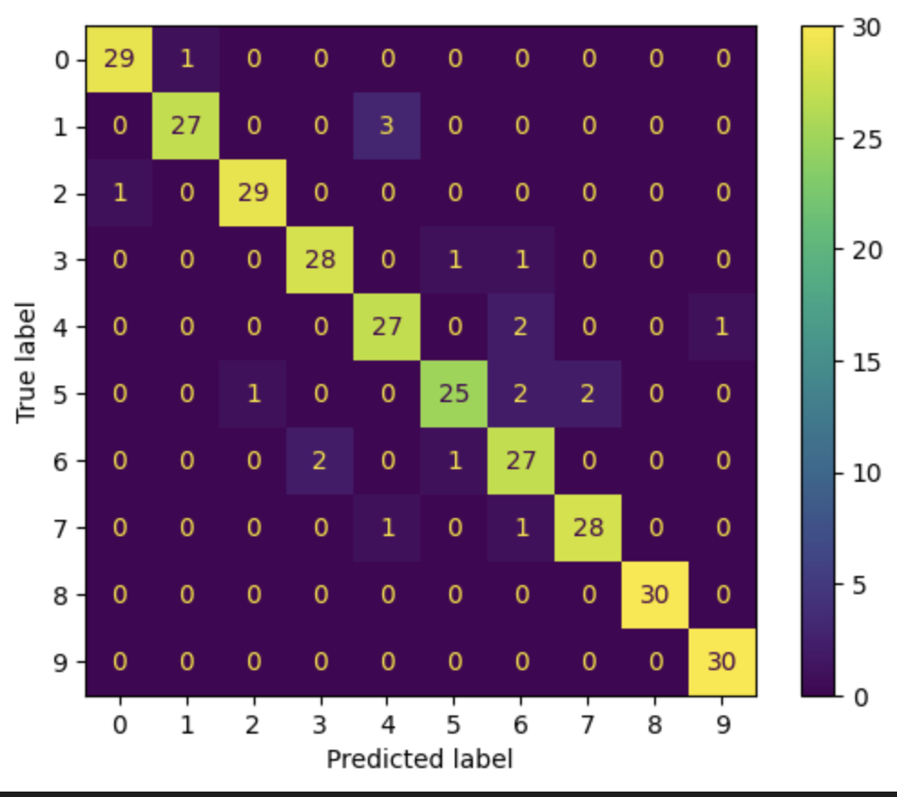
from sklearn.metrics import confusion_matrix, ConfusionMatrixDisplay

M = confusion_matrix(y_labels, y_pred)
disp = ConfusionMatrixDisplay(confusion_matrix=M)

Text classification (via EfficientNet V2 S)

Setup

Classify 10 classes in Animal image dataset using EfficientNet V2 model
Use GPU for training
Input : image in size (224, 224, 3)
- (230, 230) -> random rotation, clop, horizontal flip, vertical flip, nomralize -> train
- normalize -> test
Output : 10 classes (0-9)
Batch size is 32
from 2,000 image splited into
1. 1,400 of train
2. 300 of validation
3. 300 of test

Model arch.

use pretrained weight from ImageNet-1000

import torchvision
pretrained_weight = torchvision.models.EfficientNet_V2_S_Weights.IMAGENET1K_V1

use EfficientNet V2 size S

model = torchvision.models.efficientnet_v2_s(weights = pretrained_weight)
model.classifier[1] = nn.Linear(1280, 10)
model.to(device)

Total parameters = 20,190,298

Training

criterion : nn.CrossEntropyLoss()
optimizer : torch.optim.SGD(model.parameters(), lr=1e-2, momentum=0.9)
scheduler : torch.optim.lr_scheduler.StepLR(optimizer, step_size=7, gamma=0.5)

Training result

Metrics

Accuracy
Precision
Recall
F1

Evaluation (confusion matrix)

Week 5

Image task

classification
detection
semantic segmentation
panoptic segmentation
- segmentation + object detection

Model explanation

GradCAM Technique

RNN (Recurrent Nueral Network)

Autoregressive model
$X_t = c+\sum_i\omega X_{t-i}$
input
1. Current features ($X_t$)
2. Previous magical number ($S_{t-1}$)
output
1. Next state value ($X_{t+1}$)
caution
- BPTT : Back Propogation Through Time -> Gradient Vanishing ß

LSTM (Long-short term memory)

avoid Gradient Vanishing
3 parts
1. input gate : input $X_t$
2. output gate : predict $X_{t+1}$
3. forget gate : to make decision how much historical info. impact
input
1. $X_t$
2. short term(last $X$), long term memory
output
1. $X_{t+1}$
2. short term(last $X$), long term memory

GRU (Gated Recurrent Nueral Network)

LSTM which smaller
input
1. $C_{t-1}$
2. $X_t$
output
1. $X_{t+1}$

Attention

to fix : normal RNN can't handle long output (e.g. ~1000 words to translate) b.s. Bottle neck issue
Main idea : use all embedded vectors instead of one
- use Attention mechanism -> weighed sum which attention score(learnable parameters)
  - $C_i = \sum_ja_{i,j}h_j$ which $C_i$ is context vector(like embedded vector in RNN)
type of attention
1. additive attention
2. multiplication attention
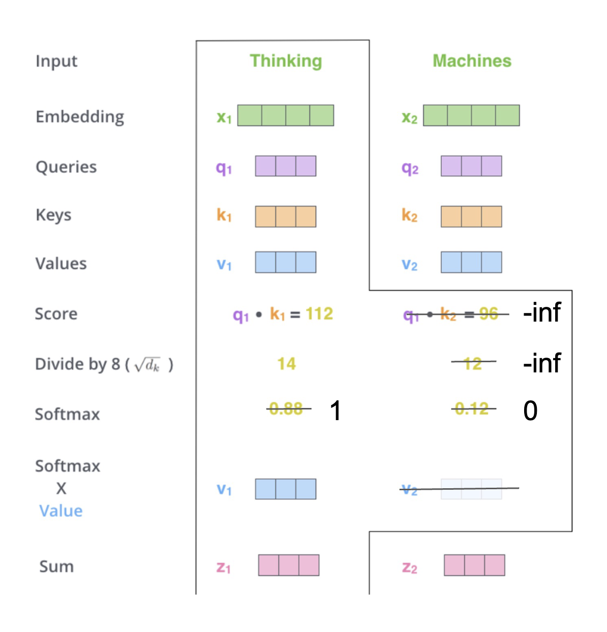
3. self-attention
  - e.g. "It's a dog" and "It's a cat", "It" is not refer to the same meaning -> we compare ourself to other again(KV attention) -> enrich meaning
4. key value attention
  - Query : what's we want to know
  - Key : index of data
  - Value : embedded vector
  - Scale dot-product formular : $\text{Attention}(Q,V,K) = \text{Softmax}(\frac{QK^T}{\sqrt{d_k}}V)$
    - $\sqrt{d_k}$ to scale number with its dimension

Transformer

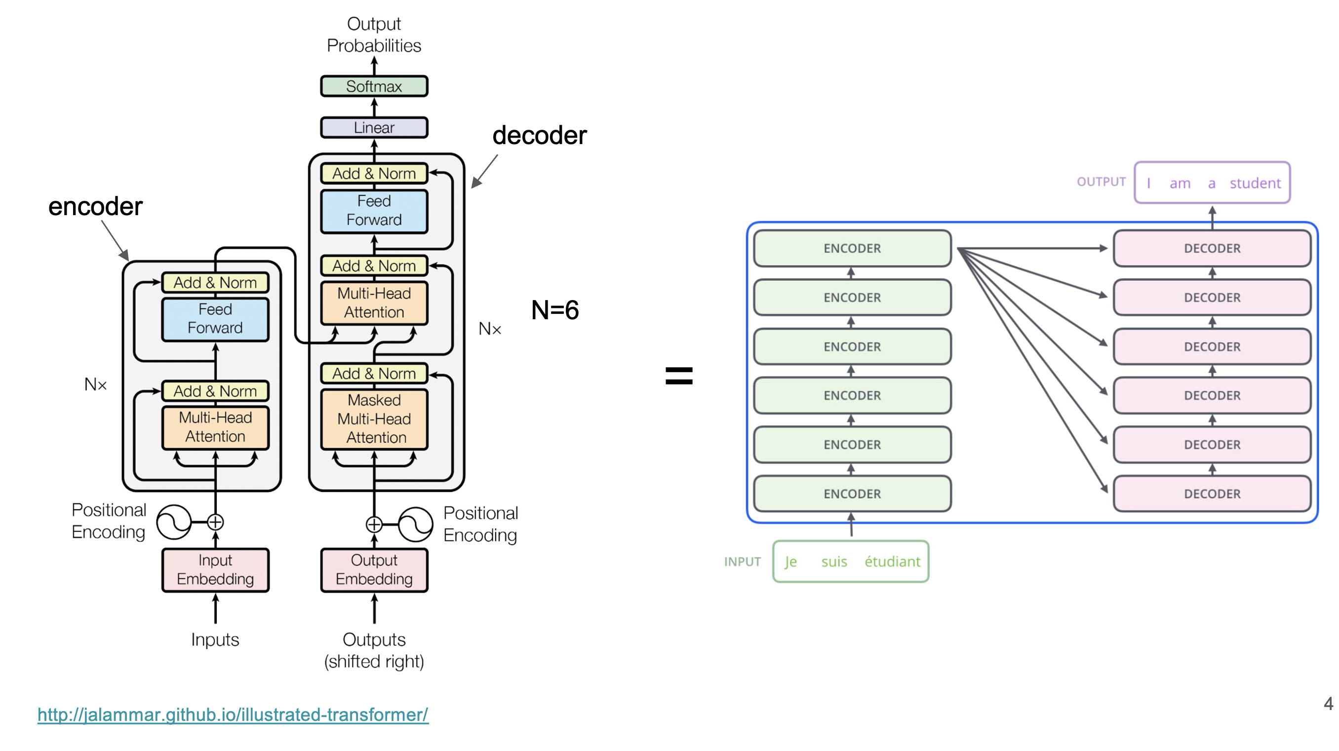
Only Attention, without RNN
transformer-based model
1. Decoder-based model : GPT
2. Encoder-based model : BERT
3. Encoder & Decoder : BART

Adapt to Image field -> ViT (Visual Transformer)

split image into smaller grid
feed like a word (act like describe each grid with image)
use transformer encoder side

When to use which

Text generation -> GPT
Text classification -> BERT

Oil and Gold

huggingface

Model monitoring

ML Flow
- traditional ML model
TensorBoard
- deep learning model
Weights & Biases
- deep learning and traditional ML model
- required API key

ML Flow (logging and monitoring)

installing

pip install mlflow --quiet --use-deprecated=legacy-resolver

import mlflow

# start logging
local_registry = 'sqlite:///mlruns.db'
mlflow.set_tracking_uri(local_registry)
exp_id = mlflow.set_experiment('my_exp')

# logging parameter
mlflow.log_param('param1', 1)

# logging metric
mlflow.log_metric('metric1', 0.5)

# logging model
mlflow.pytorch.log_model(model, 'model')

# search run
best_model_df = mlflow.search_runs(order_by=['metrics.metric1 DESC'], max_results=5)

# get model
best_model = mlflow.pytorch.load_model(best_model_df.iloc[0].artifact_uri)

# MLflow UI
!mlflow ui
'''
access through link http://localhost:5000
'''
!pip install pyngrok --quiet

from pyngrok import ngrok
ngrok.kill()

#Setting the authtoken (optional)
#Get your authtoken from https://ngrok.com/
NGROK_AUTH_TOKEN = '2TsHdd1tFmtp1cSZzWaNda1Kv9l_3b6htuCHs43LHyK2YQgVH' # Enter your authtoken
ngrok.set_auth_token(NGROK_AUTH_TOKEN)

# Open an HTTPs tunnel on port 5000 for http://localhost:5000
ngrok_tunnel = ngrok.connect(addr='5000', proto='http', bind_tls=True)
print("MLflow Tracking UI: ", ngrok_tunnel.public_url)

Exam

ML
pipeline
ML flow

Example Assignment 5-1

Reference

class github

jirayuwat12/2110446-DS-and-DE

2110446-DS-and-DE

Acknowledgement

1st week

key pandas command

Assignment 1

2nd week

Week 3

AI

Supervise learning (Predictive task)

Type of problem

Unsupervise learning

Impurity reduction

Tree visualization

Regularization

Dicision tree classifier

Bagging ( Bootstrap Aggregation )

Boosting

Random forest classifier

hyperparameters

Feature selection from tree (feature importance) with shortcut

Linear regression

Week 4

kNNs

Caution

GridSearchCV

RandomizeSearchCV

Save & Load model

Pipelining

Neural Network

Weight updating

CNN

example

Use case

Image classification (via CNN)

Setup

Model arch.

Training

Training result

Metrics

Evaluation (confusion matrix)

Text classification (via EfficientNet V2 S)

Setup

Model arch.

Training

Training result

Metrics

Evaluation (confusion matrix)

Week 5

Image task

Model explanation

RNN (Recurrent Nueral Network)

LSTM (Long-short term memory)

GRU (Gated Recurrent Nueral Network)

Attention

Transformer

Adapt to Image field -> ViT (Visual Transformer)

When to use which

Oil and Gold

Model monitoring

ML Flow (logging and monitoring)

Exam

Reference