How to Spot a (Russian) Troll

Student name: James M. Irving, Ph.D.
Student pace: Full Time
Instructor name: Brandon Lewis, Jeff Herman

Goal:

To create a deep-learning Natural Language Processing neural network that can analyze the language content of a Tweet to determine if the tweet was written by an authentic user or a Russian Troll.

Methods Overview:

Analysis Framework

We will be using the OSEMN framework (outlined in brief below)
- Obtain
  - Extract new Twitter control tweets.
  - Merge with Kaggle/FiveThirtyEight dataset
- Scrub
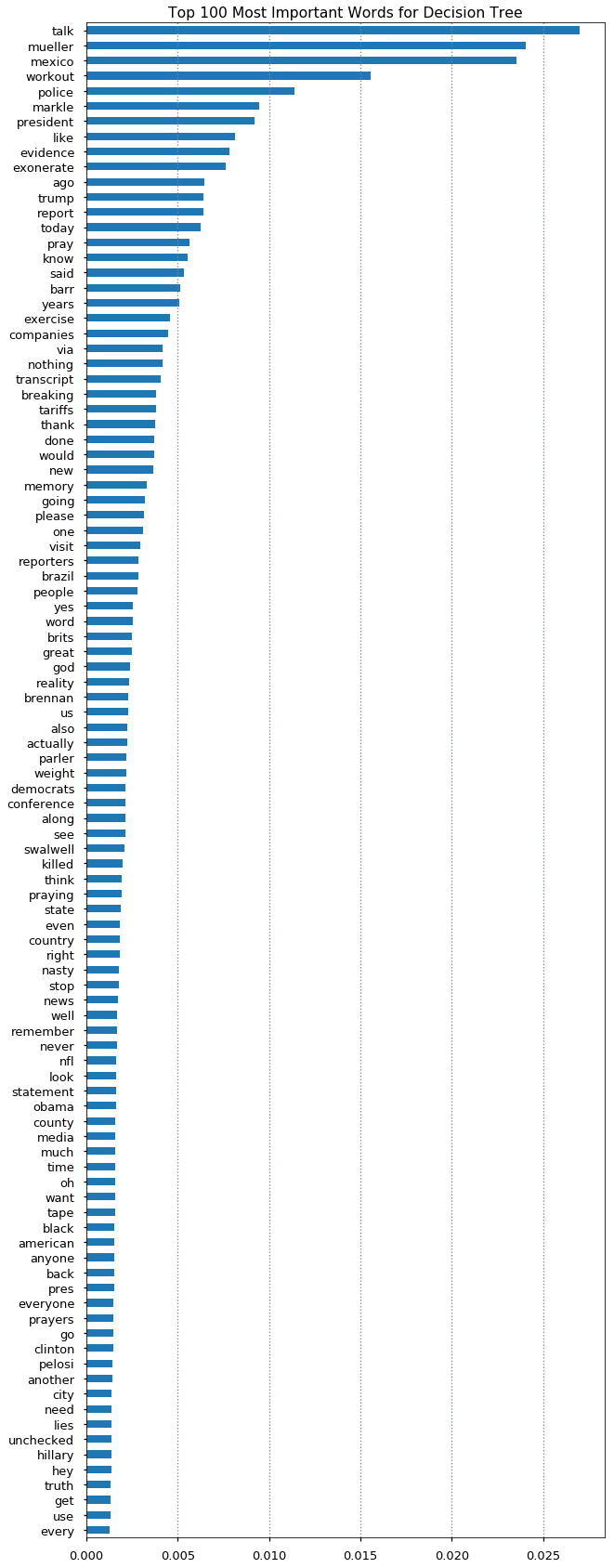
  - Remove hashtags, mentions, misleading common terms (discovered by feature importance in Decision Tree Classifier.
- Explore
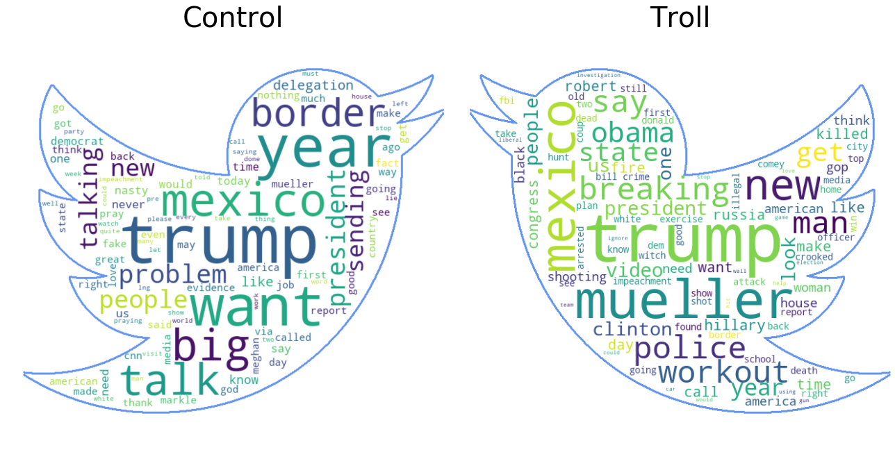
  - WordClouds for tokenized, stop-word removed text.
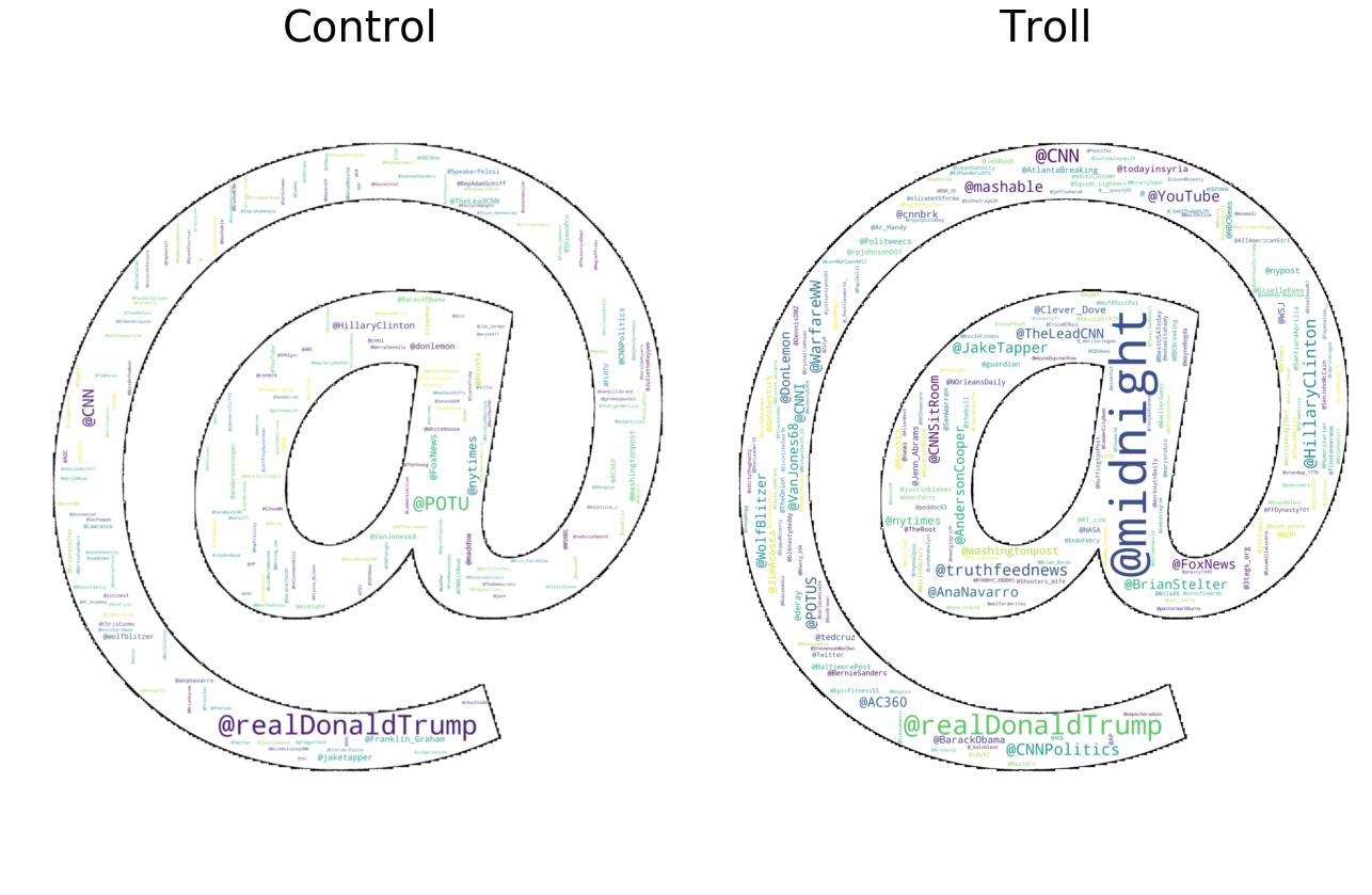
    - Also for hashtags, mentions
    - Bigrams & Pointwise Mutual Information Score
    - Sentiment Analysis
- Model
  - Logistic Regression
  - Decision Tree Classifier
  - Random Forests Classifier
  - Artificial Neural Networks (3 vers)
- Interpret
  - Summary
  - Future Directions

Data Sources

Russian Troll Tweets

We started with a dataset of 3 Million Tweets sent from 2,752 Twitter accounts connected to the "Internet Research Agency," a Russian-Troll farm that was part of The Mueller Investigation's February 2018 indictments. The tweets cover a range from February 2012 to May 2018, with the majority published from 2015-2017. > - The tweets published on Kaggle by FiveThirtyEight and were originally collected by Clemson University researchers, Dr. Darren Linvill and Dr. Patrick Warren, using custom searches using Social-Studio software licensed by Clemson University.

> - Their analysis on the various tactics used and the various social groups that were targeted by the trolls is detailed in their manuscript "Troll Factories: The Internet Research Agency and State-Sponsored Agenda Building" published in July of 2018.

Appropriate Control Tweets

However, since the goal is to produce a machine learning model that can accurately classify if a tweet came from an authentic user or a Russian troll, we needed to acquire a set of control tweets from non-trolls.

We used Tweepy to to extract a set of control tweets from the twitter api. - Our goal was to extract tweets from the same time period as the troll tweet dataset, matching the top 20 hashtags(#) and mentions(@).

- However, due to limitations of the Twitter API (including the inability to search for specific date ranges) we extracted present-day tweets directed at the top 40 most-frequent mentions (@s) from the troll Tweets.
- (The top 20 hashtags contained many generic topics (#news, #sports) that would not be proper controls for the language content of the troll tweets.)

Our newly extracted control dataset is comprised of:
- 39,086 tweets ranging from 05/24/19 to 06/03/19.

We do not have equal number of troll tweets and new tweets

We will resample from the troll tweets to meet the # of new controls.

Original Troll Dataset Features & Observations

For our analyses, we will be focusing strictly on the language of the tweets, and none of the other characteristics int he dataset.

Observations on the Troll Tweet Dataset

Dataset is comprised of 2,973,371 tweets. - Target Tweet Text to Analyze is in Content

Thoughts on specific features:
- language
  - There are 56 unique languages.
  - 2.1 million are English (71.6%), 670 K are in Russian, etc.
  - Drop all non-English tweets.
- retweet
  - 1.3 million entries are retweets (44.1 % )
  - Since this analysis will use language content to predict author, retweets are not helpful.
  - Retweets were not written by the account's author and should be not considered.
  - Drop all retweets
Final Troll Tweet Summary:
- After dropping non-English tweets and retweets, there are 1,272,848 Russian-Troll tweets.

OBTAIN:

Control Tweet Extract with TwitterAPI

See Notebook "student_JMI_twitter_extraction.ipynb" for the extraction of control tweets to match the Troll tweets.

Combining & Sampling Original Troll Tweets and with Newly-Harvested Control Tweets

.dataframe tbody tr th {
    vertical-align: top;
}

.dataframe thead th {
    text-align: right;
}

</style>

	external_author_id	author	content	region	language	publish_date	following	followers	updates	post_type	account_type	retweet	account_category	troll_tweet
date_published
2017-10-01 19:58:00	9.060000e+17	10_GOP	"We have a sitting Democrat US Senator on tria...	Unknown	English	10/1/2017 19:58	1052	9636	253	NaN	Right	0	RightTroll	1
2017-10-01 22:43:00	9.060000e+17	10_GOP	Marshawn Lynch arrives to game in anti-Trump s...	Unknown	English	10/1/2017 22:43	1054	9637	254	NaN	Right	0	RightTroll	1
2017-10-01 23:52:00	9.060000e+17	10_GOP	JUST IN: President Trump dedicates Presidents ...	Unknown	English	10/1/2017 23:52	1062	9642	256	NaN	Right	0	RightTroll	1

There were 832208 unique hashtags and 673442 unique @'s

.dataframe tbody tr th {
    vertical-align: top;
}

.dataframe thead th {
    text-align: right;
}

</style>

	tags	% Total
#news	118624	14.254129
#sports	45544	5.472670
#politics	37452	4.500317
#world	27077	3.253634
#local	23130	2.779353
#TopNews	14621	1.756893
#health	10328	1.241036
#business	9558	1.148511
#BlackLivesMatter	8252	0.991579
#tech	7836	0.941592

.dataframe tbody tr th {
    vertical-align: top;
}

.dataframe thead th {
    text-align: right;
}

</style>

	ats	% Total
@midnight	6691	0.993553
@realDonaldTrump	3532	0.524470
@WarfareWW	1529	0.227043
@CNN	1471	0.218430
@HillaryClinton	1424	0.211451
@POTUS	1035	0.153688
@CNNPolitics	948	0.140769
@FoxNews	930	0.138097
@mashable	740	0.109883
@YouTube	680	0.100974

(None, None)

SCRUB:

Text Processing: tokenizing, removing stopwords, urls, hashtags

Using RegularExpressions to extract and replace Urls, Hashtags, and Mentions

URLs, hasthtags, mentions were already removed.
- hashtags and mentions are in content_hashtags,content_mentions
Cleaned data columns are:
- content_min_clean: only RT headers and urls have been removed.
- content: RT headers, urls, hashtags, mentions were all removed.

ADDRESSING THE "RT" ISSUE

Summary: many messages in both the troll tweets and new control tweets are prepended with "RT".
- Some are RT @handle: others are just RT handle:, but SOME are using RT internally as an abbreviation for the idea of a retweet, not as an indicator that the current message is a retweet.

Reference Article from 2014 re: the usage of RT and more modern methods of reatweeting.
According to this article, using "RT @Username:" in an anachronism that has been replaced by an automated retweet function, but that many die-hard old school twitter users still prefer to do it the manual way.
Therefore, by filtering out tweets marked as officially retweeted by the Twitter API, but keeping tweets thats were manually retweeted using "RT @handle:", can produce a sort of sampling error.
- That being said, if someone is taking the effort to manually type the origin and quote, that level of effort, in my opinion, still is a reasonable metric to use to separate out these tweets from the auto-retweeted tweets.
HOWEVER: there is still the issue of what effect this has on the dataset.
My proposed solution:
1. take current df['content'] column and change it to df['content_raw'] (so that it is no longer used by the following code)
2. create a new df['content_min_clean'] column that uses regexp to remove all RT @handle: and RT handle: from the df['raw'] column and all URL links, but keeps mentions and hashtags
  - Use for some vectorized analyses
3. Create a new hashtags and mentions columns that will find and save any handles and hashtags from anywhere in the NEW RT @mention:-removed content.
  - This means that any hashtags that represent the original source and are pre-pended to the message will NOT be included, but any other mentions WILL be included.

Resampling Troll Tweets to Match Number of Control Tweets

Since there are many fewer new tweets, we will sample the same # from the larger Troll tweet collection.
An issue to be reconsidered in future analyses is how to resample in a way that ensures that chosen troll tweets will be as close to the control tweets as the dataset allows.
- In other words, making sure that if a term appears in the new control tweets, that we purposefully include matching tweets in our resampled troll tweets.

Revisiting Data to be Included/Excluded from the Analysis.

This may or may not be necessary, so saving it as markdown for now until revisiting the word frequency results.

## TO CHECK FOR STRINGS IN TWO DATAFRAMES:
def check_dfs_for_exp_list(df_controls, df_trolls, list_of_exp_to_check):
    import bs_ds as bs
    list_of_results=[['Term','Control Tweets','Troll Tweets']]
    for exp in list_of_exp_to_check:
        num_control = len(df_controls.loc[df_controls['content_min_clean'].str.contains(exp)])
        num_troll = len(df_trolls.loc[df_trolls['content_min_clean'].str.contains(exp)])
        list_of_results.append([exp,num_control,num_troll])
    df_results = bs.list2df(list_of_results, index_col='Term')
    return df_results

## TO CHECK FOR STRINGS IN TWO GROUPS FROM ONE DATAFRAME 
def check_df_groups_for_exp(df_full, list_of_exp_to_check, check_col='content_min_clean', groupby_col='troll_tweet', group_dict={0:'Control',1:'Troll'}):      
    """Checks `check_col` column of input dataframe for expressions in list_of_exp_to_check and 
    counts the # present for each group, defined by the groupby_col and groupdict. 
    Returns a dataframe of counts."""
    import bs_ds as bs
    list_of_results = []      

    header_list= ['Term']
    [header_list.append(x) for x in group_dict.values()]
    list_of_results.append(header_list)
    
    for exp in list_of_exp_to_check:
        curr_exp_list = [exp]
        
        for k,v in group_dict.items():
            df_group = df_full.groupby(groupby_col).get_group(k)
            curr_group_count = len(df_group.loc[df_group[check_col].str.contains(exp)])
            curr_exp_list.append(curr_group_count)
        
        list_of_results.append(curr_exp_list)
        
    df_results = bs.list2df(list_of_results, index_col='Term')
    return df_results

## CHECKING WORD OCCURANCES 
# Important Features from Decision Tree Classificaiton: verify if they are present in Troll and Controll Tweets
list_of_exp_to_check = ['[Pp]eggy','[Nn]oonan','[Mm]exico','nasty','impeachment','[mM]ueller']
df_compare = check_df_groups_for_exp(df_full, list_of_exp_to_check)

The troll_tweet classes are imbalanced.
There are 1272847 troll tweets and 39086 control tweets

## REMOVE MISLEADING FREQUENT TERMS
import bs_ds as bs
# Removing Peggy Noonan since she was one of the most important words and theres a recent news event about her
list_to_remove =['[Pp]eggy','[Nn]oonan']

for exp in list_to_remove:
    df_full['content'].loc[df_full['content_min_clean'].str.contains(exp)]=np.nan
    df_full.dropna(subset=['content'],inplace=True)

print("New Number of Control Tweets=",len(df_full.loc[df_full['troll_tweet']==0]))
print(f"New Number of Troll Tweets=",len(df_full.loc[df_full['troll_tweet']==1]))
# Re-check for list of expressions
df_compare = check_df_groups_for_exp(df_full, list_of_exp_to_check)
df_compare.style.set_caption('Full Dataset Expressions')

New Number of Control Tweets= 38094
New Number of Troll Tweets= 1272760

EXPLORE

Generating Frequency Distribtuions

import nltk
import string
from nltk import word_tokenize

def get_group_texts_tokens(df_small, groupby_col='troll_tweet', group_dict={0:'controls',1:'trolls'}, column='content_stopped'):
    from nltk import regexp_tokenize
    pattern = "([a-zA-Z]+(?:'[a-z]+)?)"
    text_dict = {}
    for k,v in group_dict.items():
        group_text_temp = df_small.groupby(groupby_col).get_group(k)[column]
        group_text_temp = ' '.join(group_text_temp)
        group_tokens = regexp_tokenize(group_text_temp, pattern)
        text_dict[v] = {}
        text_dict[v]['tokens'] = group_tokens
        text_dict[v]['text'] =  ' '.join(group_tokens)
            
    print(f"{text_dict.keys()}:['tokens']|['text']")
    return text_dict

# Function will return a dictionary of all of the text and tokens split by group
TEXT = get_group_texts_tokens(df_small,groupby_col='troll_tweet', group_dict={0:'controls',1:'trolls'}, column='content_stopped')

# TEXT[Group][Text-or-Tokens]
TEXT['trolls']['tokens'][:10]

dict_keys(['controls', 'trolls']):['tokens']|['text']





['building',
 'collapses',
 'mexico',
 'city',
 'following',
 'magnitude',
 'earthquake',
 'current',
 'scene',
 'mexico']

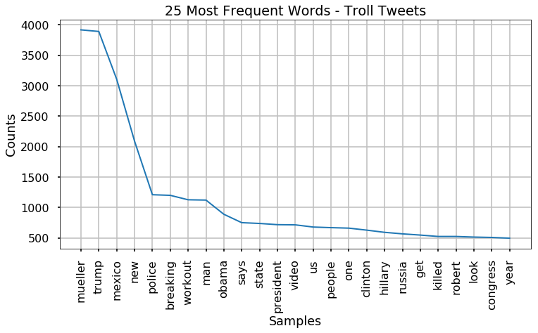
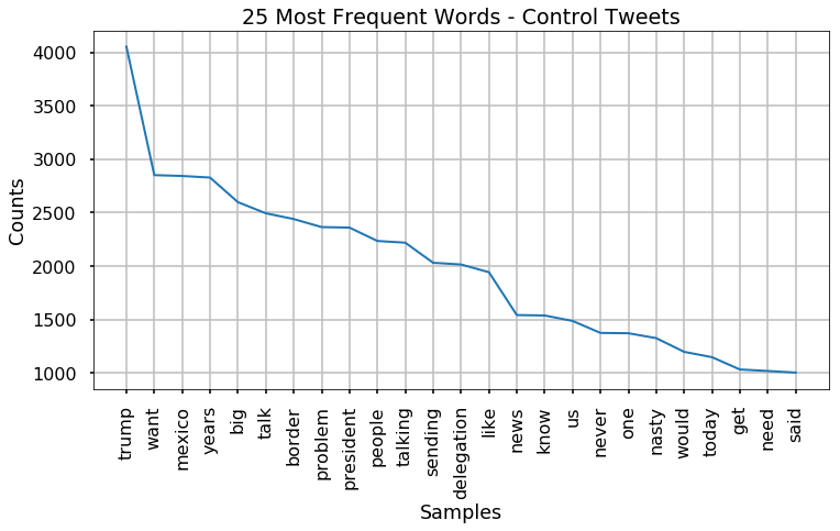
from nltk import FreqDist

TEXT = get_group_texts_tokens(df_small)

freq_trolls = FreqDist(TEXT['trolls']['tokens'])
freq_controls = FreqDist(TEXT['controls']['tokens'])

df_compare=pd.DataFrame()
df_compare['Troll Words'] = freq_trolls.most_common(25)
df_compare['Control Words'] = freq_controls.most_common(25)
display(df_compare)

# print(freq_controls.most_common(50))

dict_keys(['controls', 'trolls']):['tokens']|['text']

.dataframe tbody tr th {
    vertical-align: top;
}

.dataframe thead th {
    text-align: right;
}

</style>

	Troll Words	Control Words
0	(mueller, 3919)	(trump, 4053)
1	(trump, 3893)	(want, 2851)
2	(mexico, 3108)	(mexico, 2843)
3	(new, 2091)	(years, 2828)
4	(police, 1210)	(big, 2598)
5	(breaking, 1200)	(talk, 2494)
6	(workout, 1127)	(border, 2440)
7	(man, 1122)	(problem, 2365)
8	(obama, 889)	(president, 2360)
9	(says, 751)	(people, 2235)
10	(state, 738)	(talking, 2219)
11	(president, 718)	(sending, 2031)
12	(video, 715)	(delegation, 2015)
13	(us, 679)	(like, 1943)
14	(people, 669)	(news, 1542)
15	(one, 661)	(know, 1538)
16	(clinton, 628)	(us, 1487)
17	(hillary, 592)	(never, 1375)
18	(russia, 567)	(one, 1372)
19	(get, 547)	(nasty, 1326)
20	(killed, 524)	(would, 1198)
21	(robert, 524)	(today, 1148)
22	(look, 514)	(get, 1033)
23	(congress, 508)	(need, 1019)
24	(year, 496)	(said, 1004)

# pause

Generating WordClouds

Wordclouds for Hashtags

Wordclouds for @'s

Creating Bigrams and PMI scores

Bigrams

Control Tweet Bigrams

	Frequency
Bigram
('border', 'problem')	0.00571695
('big', 'delegation')	0.00569424
('talking', 'years')	0.0056914
('sending', 'big')	0.00568572
('talk', 'border')	0.00568572
('years', 'want')	0.00568572
('delegation', 'talk')	0.00568288
('mexico', 'sending')	0.00568288
('problem', 'talking')	0.00568288
('fake', 'news')	0.00184509
('meghan', 'markle')	0.00183658
('markle', 'nasty')	0.00167761
('never', 'called')	0.00156975
('called', 'meghan')	0.00155555
('want', 'mexico')	0.00131143
('news', 'media')	0.00120641
('got', 'caught')	0.00118086
('caught', 'cold')	0.00117518
('made', 'fake')	0.00116383
('president', 'trump')	0.00116099
('media', 'got')	0.00115815
('nasty', 'made')	0.00115815
('eyes', 'ears')	0.00112693
('pres', 'trump')	0.00111841
('evidence', 'eyes')	0.00111557

	Frequency
Bigram
('new', 'mexico')	0.00338416
('robert', 'mueller')	0.00168116
('witch', 'hunt')	0.00112805
('crooked', 'mueller')	0.000967941
('donald', 'trump')	0.000949747
('year', 'old')	0.000949747
('president', 'trump')	0.000822386
('ignores', 'mueller')	0.000785998
('grand', 'jury')	0.000775081
('coup', 'using')	0.000753248
('approval', 'tanks')	0.000724137
('tanks', 'gt')	0.000724137
('mueller', 'credibility')	0.000698665
('rosenstein', 'mueller')	0.000698665
('deep', 'state')	0.000651359
('lose', 'weight')	0.000644081
('special', 'counsel')	0.000618609
('credibility', 'think')	0.00058222
('mexico', 'border')	0.000571304
('white', 'house')	0.000567665
('attempts', 'coup')	0.000556748
('gt', 'attempts')	0.000556748
('mueller', 'witch')	0.000505804
('hillary', 'clinton')	0.000491248
('crimes', 'obama')	0.000473054

Pointwise Mutual Information Score

Interesting, but heavily influenced by the different time periods.

Control Tweets

	PMI Score
Bigrams
('disappearance', 'connecticut')	16.1045
('glen', 'tyrone')	16.1045
('uscis', 'ignor')	16.1045
('advisers', 'departing')	15.8414
('babyhands', 'mcgrifter')	15.8414
('bryan', 'stevenson')	15.8414
('computer', 'intrusions')	15.8414
('grounding', 'airline')	15.8414
('haberman', 'sycophancy')	15.8414
('intimidating', 'construc')	15.8414
('rio', 'grande')	15.8414
('capone', 'vault')	15.619
('hs', 'bp')	15.619
('partnership', 'racing')	15.619
('racing', 'airs')	15.619
('riskier', 'bureaucracy')	15.619
('rweet', 'apprec')	15.619
('unprepared', 'temperamentally')	15.619
('vr', 'arcade')	15.619
('bites', 'dust')	15.5784

	PMI Score
Bigrams
('cessation', 'hostilities')	15.7461
('dunkin', 'donuts')	15.7461
('lena', 'dunham')	15.7461
('notre', 'dame')	15.7461
('snoop', 'dogg')	15.7461
('boko', 'haram')	15.4831
('lectric', 'heep')	15.4831
('nagorno', 'karabakh')	15.4831
('kayleigh', 'mcenany')	15.2607
('otto', 'warmbier')	15.2607
('allahu', 'akbar')	15.0681
('elon', 'musk')	15.0681
('ez', 'zor')	15.0681
('peanut', 'butter')	15.0681
('palo', 'alto')	14.8981
('tomi', 'lahren')	14.8981
('trey', 'gowdy')	14.8981
('betsy', 'devos')	14.8457
('caitlyn', 'jenner')	14.7753
('cranky', 'senile')	14.7461

Sentiment Analysis with VADER

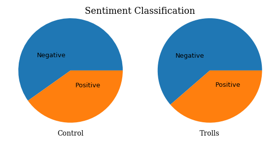
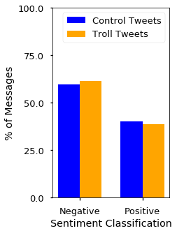
RESULTS OF SENTIMENT ANALYSIS BINARY CLASSIFICATION:
 ------------------------------------------------------------
	Normalized Troll Classes:
 pos    0.613535
neg    0.386465
Name: sentiment_class, dtype: float64

	Normalized Control Classes:
 pos    0.598126
neg    0.401874
Name: sentiment_class, dtype: float64

MODEL

BUILDING THE INITIAL MODELS

Logistic Regression

Summary Table of Clocked Processes

Lap #	Start Time	Duration	Label
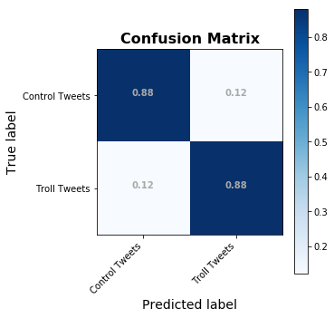
TOTAL	09/11/19 - 12:00:27 PM	0 min, 0.945 sec	LogisticRegression complete.

               precision    recall  f1-score   support

           0       0.88      0.88      0.88      7552
           1       0.88      0.88      0.88      7551

   micro avg       0.88      0.88      0.88     15103
   macro avg       0.88      0.88      0.88     15103
weighted avg       0.88      0.88      0.88     15103

Train Accuracy:  0.9390843738176314
Test Accuracy:  0.8788320201284513

INITIAL MODEL SUMMARY: Logistic Regression

Accuracy:
- 0.938 for train set
- 0.875 for test set
Recall/Precision/F1-scores all around 0.87
Duration:
- 0.78 sec

DecisionTreeClassifier

Summary Table of Clocked Processes

Lap #	Start Time	Duration	Label
TOTAL	09/11/19 - 12:00:28 PM	0 min, 20.204 sec

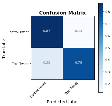
Train Accuracy:  0.9390843738176314
Test Accuracy:  0.8273852876911871

Plotting Feature Importance

Random Forests Classifier

Summary Table of Clocked Processes

Lap #	Start Time	Duration	Label
TOTAL	09/11/19 - 12:00:50 PM	2 min, 36.929 sec	Accuracy:0.8273852876911871

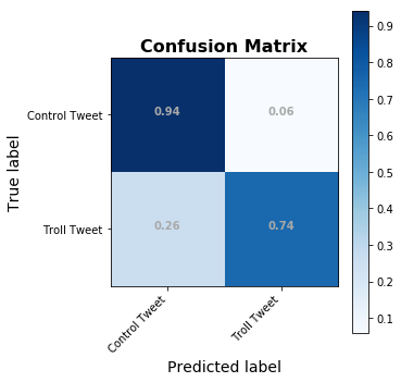
              precision    recall  f1-score   support

           0       0.79      0.94      0.86      7552
           1       0.93      0.74      0.83      7551

   micro avg       0.84      0.84      0.84     15103
   macro avg       0.86      0.84      0.84     15103
weighted avg       0.86      0.84      0.84     15103

Train Accuracy:  0.9390843738176314
Test Accuracy:  0.8428126862212806

Keras Model 1: creating a Text Classification Neural Network in Keras

Using CountVectorized data generated above

from keras import models, layers, optimizers
input_dim = X_train.shape[1]
# input_dim = sequences_train.shape[1]
print(input_dim)

model1 = models.Sequential()
# model.add(layers.Embedding)

model1.add(layers.Dense(10, input_dim= input_dim, activation='relu'))
model1.add(layers.Dense(1, activation='sigmoid'))

model1.compile(loss='binary_crossentropy',optimizer="adam",metrics=['accuracy'])
model1.summary()

30191
WARNING:tensorflow:From C:\Users\james\Anaconda3\envs\learn-env-ext\lib\site-packages\tensorflow\python\framework\op_def_library.py:263: colocate_with (from tensorflow.python.framework.ops) is deprecated and will be removed in a future version.
Instructions for updating:
Colocations handled automatically by placer.
_________________________________________________________________
Layer (type)                 Output Shape              Param #   
=================================================================
dense_1 (Dense)              (None, 10)                301920    
_________________________________________________________________
dense_2 (Dense)              (None, 1)                 11        
=================================================================
Total params: 301,931
Trainable params: 301,931
Non-trainable params: 0
_________________________________________________________________



--- CLOCK STARTED @:    09/11/19 - 12:03:27 PM           Label: starting keras .fit --- 
WARNING:tensorflow:From C:\Users\james\Anaconda3\envs\learn-env-ext\lib\site-packages\tensorflow\python\ops\math_ops.py:3066: to_int32 (from tensorflow.python.ops.math_ops) is deprecated and will be removed in a future version.
Instructions for updating:
Use tf.cast instead.
Train on 52860 samples, validate on 7552 samples
Epoch 1/10
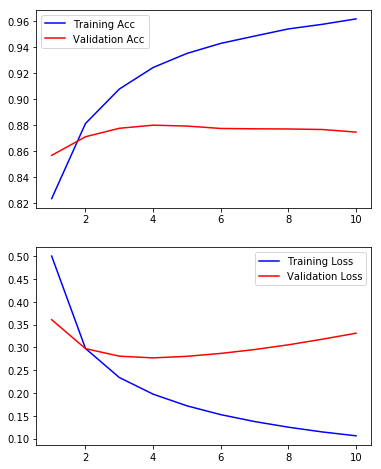
52860/52860 [==============================] - 22s 407us/step - loss: 0.5001 - acc: 0.8236 - val_loss: 0.3608 - val_acc: 0.8567
Epoch 2/10
52860/52860 [==============================] - 20s 384us/step - loss: 0.2977 - acc: 0.8812 - val_loss: 0.2973 - val_acc: 0.8710
Epoch 3/10
52860/52860 [==============================] - 20s 387us/step - loss: 0.2340 - acc: 0.9076 - val_loss: 0.2808 - val_acc: 0.8775
Epoch 4/10
52860/52860 [==============================] - 22s 414us/step - loss: 0.1975 - acc: 0.9242 - val_loss: 0.2770 - val_acc: 0.8799
Epoch 5/10
52860/52860 [==============================] - 23s 431us/step - loss: 0.1719 - acc: 0.9350 - val_loss: 0.2805 - val_acc: 0.8792
Epoch 6/10
52860/52860 [==============================] - 22s 417us/step - loss: 0.1526 - acc: 0.9427 - val_loss: 0.2868 - val_acc: 0.8774
Epoch 7/10
52860/52860 [==============================] - 25s 470us/step - loss: 0.1375 - acc: 0.9483 - val_loss: 0.2953 - val_acc: 0.8771
Epoch 8/10
52860/52860 [==============================] - 23s 439us/step - loss: 0.1251 - acc: 0.9538 - val_loss: 0.3057 - val_acc: 0.8770
Epoch 9/10
52860/52860 [==============================] - 22s 425us/step - loss: 0.1147 - acc: 0.9573 - val_loss: 0.3180 - val_acc: 0.8766
Epoch 10/10
52860/52860 [==============================] - 24s 453us/step - loss: 0.1062 - acc: 0.9615 - val_loss: 0.3311 - val_acc: 0.8746
--- TOTAL DURATION   =  3 min, 43.946 sec ---

Summary Table of Clocked Processes

Lap #	Start Time	Duration	Label
TOTAL	09/11/19 - 12:03:27 PM	3 min, 43.946 sec	completed 10 epochs

52860/52860 [==============================] - 19s 366us/step
Training Accuracy:0.9676125614696319
15103/15103 [==============================] - 5s 355us/step
Testing Accuracy:0.8750579354542498

Summary - Neural Network Analysis on CountVectorized Tweets

Accuracy:
- Training: 0.968
- Testing:0.880
Run time:
- 2:48 min

Keras Model 2 Adding pretrained Word2Vec embeddings

Adding Word2Vec vectorization into an embedding layer

How to get a word2vector model's vectors into a Keras Embedding Layer

https://sturzamihai.com/how-to-use-pre-trained-word-vectors-with-keras/

text_data = df_tokenize['content']
from gensim.models import Word2Vec
vector_size = 300

wv_keras = Word2Vec(text_data, size=vector_size, window=10, min_count=1, workers=4)
wv_keras.train(text_data,total_examples=wv_keras.corpus_count, epochs=10)

wv = wv_keras.wv

vocab_size = len(wv_keras.wv.vocab)
print(f'There are {vocab_size} words in the word2vec vocabulary, with a vector size {vector_size}.')

There are 801 words in the word2vec vocabulary, with a vector size 300.

https://adventuresinmachinelearning.com/word2vec-keras-tutorial/ https://machinelearningmastery.com/use-word-embedding-layers-deep-learning-keras/

# save the vectors in a new matrix
word_model = wv_keras
vector_size = word_model.wv.vectors[1].shape[0]

embedding_matrix = np.zeros((len(word_model.wv.vocab) + 1, vector_size))
for i, vec in enumerate(word_model.wv.vectors):
  embedding_matrix[i] = vec

# Get list of texts to be converted to sequences
# sentences_train =text_data # df_tokenize['tokens'].values
from keras.preprocessing.text import Tokenizer

tokenizer = Tokenizer(num_words=len(wv.vocab))
tokenizer.fit_on_texts(list(text_data)) #tokenizer.fit_on_texts(text_data)

word_index = tokenizer.index_word
reverse_index = {v:k for k,v in word_index.items()}

# return integer-encoded sentences
from keras.preprocessing import text, sequence
X = tokenizer.texts_to_sequences(text_data)
X = sequence.pad_sequences(X)

y = df_tokenize['troll_tweet'].values
# reverse_index
X_train, X_test, X_val, y_train, y_test, y_val = train_test_val_split(X, y)#, test_size=0.1, shuffle=False)

model2 = models.Sequential()

model2.add(layers.Embedding(len(wv_keras.wv.vocab)+1,
                             vector_size,input_length=X_train.shape[1],
                             weights=[embedding_matrix],trainable=False)) 
          
model2.add(layers.LSTM(300, return_sequences=False))#, kernel_regularizer=regularizers.l2(.01)))
# model1B.add(layers.GlobalMaxPooling1D())
model2.add(layers.Dense(10, activation='relu'))
model2.add(layers.Dense(1, activation='sigmoid'))

model2.compile(loss='binary_crossentropy',optimizer="adam",metrics=['accuracy'])
model2.summary()

_________________________________________________________________
Layer (type)                 Output Shape              Param #   
=================================================================
embedding_1 (Embedding)      (None, 51, 300)           240600    
_________________________________________________________________
lstm_1 (LSTM)                (None, 300)               721200    
_________________________________________________________________
dense_3 (Dense)              (None, 10)                3010      
_________________________________________________________________
dense_4 (Dense)              (None, 1)                 11        
=================================================================
Total params: 964,821
Trainable params: 724,221
Non-trainable params: 240,600
_________________________________________________________________

num_epochs = 5
history = model2.fit(X_train, y_train, epochs=num_epochs, verbose=True, validation_data=(X_val, y_val), batch_size=500)

--- CLOCK STARTED @:    09/11/19 - 12:08:20 PM           Label: starting keras .fit --- 
Train on 52860 samples, validate on 7552 samples
Epoch 1/5
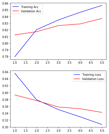
52860/52860 [==============================] - 131s 2ms/step - loss: 0.4562 - acc: 0.7795 - val_loss: 0.3929 - val_acc: 0.8124
Epoch 2/5
52860/52860 [==============================] - 127s 2ms/step - loss: 0.3790 - acc: 0.8203 - val_loss: 0.3764 - val_acc: 0.8173
Epoch 3/5
52860/52860 [==============================] - 127s 2ms/step - loss: 0.3503 - acc: 0.8348 - val_loss: 0.3578 - val_acc: 0.8264
Epoch 4/5
52860/52860 [==============================] - 120s 2ms/step - loss: 0.3292 - acc: 0.8464 - val_loss: 0.3528 - val_acc: 0.8289
Epoch 5/5
52860/52860 [==============================] - 122s 2ms/step - loss: 0.3068 - acc: 0.8568 - val_loss: 0.3420 - val_acc: 0.8371
--- TOTAL DURATION   =  10 min, 28.585 sec ---

Summary Table of Clocked Processes

Lap #	Start Time	Duration	Label
TOTAL	09/11/19 - 12:08:20 PM	10 min, 28.585 sec	completed 5 epochs

loss, accuracy = model2.evaluate(X_train, y_train, verbose=True)
print(f'Training Accuracy:{accuracy}')

loss, accuracy = model2.evaluate(X_test, y_test, verbose=True)
print(f'Testing Accuracy:{accuracy}')

52860/52860 [==============================] - 70s 1ms/step
Training Accuracy:0.8670450245977757
15103/15103 [==============================] - 20s 1ms/step
Testing Accuracy:0.8459908626911964

jmi.plot_keras_history(history)

(<Figure size 432x576 with 2 Axes>,
 array([<matplotlib.axes._subplots.AxesSubplot object at 0x000001FAF83FAA58>,
        <matplotlib.axes._subplots.AxesSubplot object at 0x000001FA851B2F28>],
       dtype=object))

model2.save('model2_emb_lstm_dense_dense.hd5',include_optimizer=True, overwrite=True)
model2.save_weights('model2_emb_lstm_dense_dense_WEIGHTS.hdf')

Keras model 3 -using keras' tokenizer to fit_on_texts+one_hot

Train, test, val split

# from sklearn.feature_extraction.text import CountVectorizer
from keras.preprocessing.text import Tokenizer, one_hot
from keras.utils.np_utils import to_categorical

from sklearn import preprocessing
from sklearn.model_selection import train_test_split

from keras import models, layers, optimizers

# df_tokenize.head()

# Define tweets to be analyzed, fit tokenizer,generate sequences
tweets = df_tokenize['content']
# num_words=len(set(tweets))
tokenizer = Tokenizer(num_words=3000)

tokenizer.fit_on_texts(tweets)
sequences = tokenizer.texts_to_sequences(tweets)

one_hot_results = tokenizer.texts_to_matrix(tweets, mode='binary')

word_index = tokenizer.word_index
reverse_index = {v:k for k,v in word_index.items()}

Test Train Split

print(one_hot_results.shape, y.shape)

(75515, 3000) (75515,)

import random, math
random.seed(42)
test_size = math.floor(one_hot_results.shape[0]*0.3)
test_index = random.sample(range(1,one_hot_results.shape[0]), test_size)

test = one_hot_results[test_index]
train = np.delete(one_hot_results, test_index, 0)
label_test = y[test_index]
label_train = np.delete(y, test_index, 0)

train.shape
train.shape[1]

model3 = models.Sequential()
model3.add(layers.Dense(50, activation='relu', input_shape=(3000,)))
model3.add(layers.Dense(25, activation='relu'))
model3.add(layers.Dense(1,activation='sigmoid'))

model3.compile(optimizer='adam', loss='binary_crossentropy',metrics=['accuracy'])
model3.summary()

_________________________________________________________________
Layer (type)                 Output Shape              Param #   
=================================================================
dense_5 (Dense)              (None, 50)                150050    
_________________________________________________________________
dense_6 (Dense)              (None, 25)                1275      
_________________________________________________________________
dense_7 (Dense)              (None, 1)                 26        
=================================================================
Total params: 151,351
Trainable params: 151,351
Non-trainable params: 0
_________________________________________________________________

clock_1hot = bs.Clock()
clock_1hot.tic()

history = model3.fit(train, label_train, epochs=10, batch_size=256, validation_data=(test, label_test))
clock_1hot.toc('')

--- CLOCK STARTED @:    09/11/19 - 12:20:30 PM --- 
Train on 52861 samples, validate on 22654 samples
Epoch 1/10
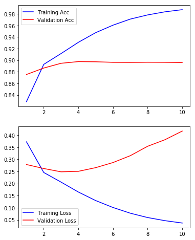
52861/52861 [==============================] - 4s 84us/step - loss: 0.3724 - acc: 0.8285 - val_loss: 0.2785 - val_acc: 0.8753
Epoch 2/10
52861/52861 [==============================] - 3s 61us/step - loss: 0.2456 - acc: 0.8929 - val_loss: 0.2620 - val_acc: 0.8865
Epoch 3/10
52861/52861 [==============================] - 3s 64us/step - loss: 0.2059 - acc: 0.9115 - val_loss: 0.2484 - val_acc: 0.8947
Epoch 4/10
52861/52861 [==============================] - 3s 66us/step - loss: 0.1648 - acc: 0.9309 - val_loss: 0.2504 - val_acc: 0.8976
Epoch 5/10
52861/52861 [==============================] - 3s 66us/step - loss: 0.1296 - acc: 0.9476 - val_loss: 0.2656 - val_acc: 0.8973
Epoch 6/10
52861/52861 [==============================] - 3s 61us/step - loss: 0.1009 - acc: 0.9606 - val_loss: 0.2867 - val_acc: 0.8964
Epoch 7/10
52861/52861 [==============================] - 3s 60us/step - loss: 0.0773 - acc: 0.9711 - val_loss: 0.3151 - val_acc: 0.8963
Epoch 8/10
52861/52861 [==============================] - 3s 60us/step - loss: 0.0594 - acc: 0.9782 - val_loss: 0.3539 - val_acc: 0.8965
Epoch 9/10
52861/52861 [==============================] - 3s 60us/step - loss: 0.0465 - acc: 0.9836 - val_loss: 0.3810 - val_acc: 0.8964
Epoch 10/10
52861/52861 [==============================] - 3s 61us/step - loss: 0.0367 - acc: 0.9873 - val_loss: 0.4169 - val_acc: 0.8959
--- TOTAL DURATION   =  0 min, 34.478 sec ---

            <tr>
                            <td id="T_27140d9e_d4b0_11e9_bdbe_f48e38b6371frow0_col0" class="data row0 col0" >TOTAL</td>
                    <td id="T_27140d9e_d4b0_11e9_bdbe_f48e38b6371frow0_col1" class="data row0 col1" >09/11/19 - 12:20:30 PM</td>
                    <td id="T_27140d9e_d4b0_11e9_bdbe_f48e38b6371frow0_col2" class="data row0 col2" >0 min, 34.478 sec</td>
                    <td id="T_27140d9e_d4b0_11e9_bdbe_f48e38b6371frow0_col3" class="data row0 col3" ></td>
        </tr>
</tbody></table>

loss, accuracy = model3.evaluate(train, label_train, verbose=True)
print(f'Training Accuracy:{accuracy}')

loss, accuracy = model3.evaluate(test, label_test, verbose=True)
print(f'Testing Accuracy:{accuracy}')

52861/52861 [==============================] - 2s 35us/step
Training Accuracy:0.990976334149251
22654/22654 [==============================] - 1s 37us/step
Testing Accuracy:0.8959124216579155

INTERPRET

Summary:
- In terms of efficiency, no model can be a simple Logistic Regression.
- Decision Trees and Random Forests did not improve performance and took significantly longer.
- In terms of accuracy, a neural network using CountVectorization with a 3 layers of neurons outperformed all other models with 90% accuracy on the testing data with a run time of 31 seconds.

- **Caveats:** - Perfect control tweets were not available due to the limitations of the twitter API. If we had access to the batch historical tweets, we may be able to better classify troll tweets, as we would be able to leave the hashtags and mentions in the body of the tweet for vectorization. - There is the possibility that the accuracy tested as-is would decrease, due to elimination of any contemporaneous events that influence tweet contents.

FUTURE DIRECTIONS

With additional time, we would have explored additional Neural Network configurations using bi-directional layers and additional Dense layers for classification.
Additional methods of words/sentence vectorization
Analysis using Named Entity Recognition with Spacey
Additional Visualization
Using the outputs of the logistic regression or neural networks with model stacking
- Adding in the other non-language characteristics of the tweets to further improve accuracy.

Summary Table of Clocked Processes

Lap #	Start Time	Duration	Label

jirvingphd/how-to-spot-a-russian-troll-tweet-mod-4-project

How to Spot a (Russian) Troll

Goal:

Methods Overview:

Analysis Framework

Data Sources

Russian Troll Tweets

Appropriate Control Tweets

Original Troll Dataset Features & Observations

Observations on the Troll Tweet Dataset

OBTAIN:

Control Tweet Extract with TwitterAPI

Combining & Sampling Original Troll Tweets and with Newly-Harvested Control Tweets

SCRUB:

Text Processing: tokenizing, removing stopwords, urls, hashtags

Using RegularExpressions to extract and replace Urls, Hashtags, and Mentions

ADDRESSING THE "RT" ISSUE

Resampling Troll Tweets to Match Number of Control Tweets

Revisiting Data to be Included/Excluded from the Analysis.

EXPLORE

Generating Frequency Distribtuions

Generating WordClouds

Wordclouds for Hashtags

Wordclouds for @'s

Creating Bigrams and PMI scores

Bigrams

Pointwise Mutual Information Score

Sentiment Analysis with VADER

MODEL

BUILDING THE INITIAL MODELS

Logistic Regression

INITIAL MODEL SUMMARY: Logistic Regression

DecisionTreeClassifier

Plotting Feature Importance

Random Forests Classifier

Keras Model 1: creating a Text Classification Neural Network in Keras

Summary - Neural Network Analysis on CountVectorized Tweets

Keras Model 2 Adding pretrained Word2Vec embeddings

How to get a word2vector model's vectors into a Keras Embedding Layer

Keras model 3 -using keras' tokenizer to fit_on_texts+one_hot

Train, test, val split

Test Train Split

INTERPRET

FUTURE DIRECTIONS