Vehicle Detection

Project for the Self-Driving Car Engineer Nanodegree Program.

Overview

In this project I created a vehicle detection and tracking pipeline with OpenCV, histogram of oriented gradients (HOG), and support vector machines (SVM). I optimized and evaluated the model on video data from a automotive camera taken during highway driving.

The goals / steps of this project are the following:

Perform a Histogram of Oriented Gradients (HOG) feature extraction on a labeled training set of images and train a classifier Linear SVM classifier
Optionally, apply a color transform and append binned color features, as well as histograms of color, to the HOG feature vector.
Note: for those first two steps, normalize the features and randomize a selection for training and testing.
Implement a sliding-window technique and use the trained classifier to search for vehicles in images.
Run the pipeline on a video stream (start with the test_video.mp4 and later implement on full project_video.mp4) and create a heat map of recurring detections frame by frame to reject outliers and follow detected vehicles.
Estimate a bounding box for vehicles detected.

Dependencies

Here are links to the labeled data for vehicle and non-vehicle examples to train the classifier. These example images come from a combination of the GTI vehicle image database, the KITTI vision benchmark suite, and examples extracted from the project video itself.

Code Description

A brief description of important steps of how (and identify where in my code) I did this project.

Histogram of Oriented Gradients (HOG)

As I have time-series data, I split it into a train set and a test set manually, around 70% and 30% respectevly. Here some information of about that:

TRAINING SET
Number of cars images =  5697
Number of no-cars images =  6278
Size =  (64, 64, 3)
Data type: uint8

TEST SET
Number of cars images =  2431
Number of no-cars images =  2690
Size =  (64, 64, 3)
Data type: uint8

For this project I create a Jupyter Notebook main.ipynb to experiment; to store the principal functions I create the my_lesson_functions.py. Is worth to note that to avoid problems with the way the different functions read images of differents formats I create my own function. This can be found as myimread() in my_lesson_functions.py. Using it, I am sure that the reading image is in RGB on a scale 0 to 255.

Coming back to the main point of rubric point, after the markdown cell with the titled "Extract features for each dataset" in the main.ipynb, the function that extract the features are called (list_extract_features()). This function receive a list of paths of each image as well as the features parameters. The code of that function is located in my_lesson_functions.py where, after changing the color space specified as the features parameters, the function that extracts the HOG features is invoked (hog_extract_features()) for every image. The hog_extract_features() use skimage.hog() function for either all channels or a specific one.

Choosing of HOG parameters

I explored different color spaces and different skimage.hog() parameters (orientations, pixels_per_cell, and cells_per_block), as well choosing between using one channel or all of them. The way I decided that parameters were training a classifier. Specifically, a Linear Suport Vector Machine (sklearn.svm.LinearSVC) with the defaults parameters. I read that the orientations parameter between 6 and 9 is a common choice so I choose 9. About pixels_per_cell, makes sense to me choose a divisor of 64 and considering the size of the car in the image I believe that 8 was a good number. In the case of cells_per_block I use 2 with not special reason. The parameters that I play most was choosing the color space and color channel. I find that using all the channels of the 'HSV' color space obtain a good result (around %96 in test accuracy).

Training the classifier using the selected HOG features,

After some experimentation training a sklearn.svm.LinearSVC with the defaults parameters, I realize that adding raw pixel intensity features and histogram features to the HOG features have better performance than using the HOG features alone. The best parameters found were spatial binning dimensions of (8,8) and 32 histograms bins.

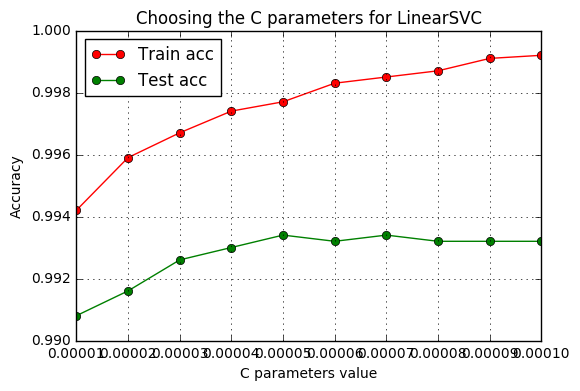
The features of the training examples were previously scaled to have 0 mean and unit variance. The scaler obtained was used to scale the test features. As the main parameter of a linear SVM is the penalty parameter C of the error term, I code in a loop, a training with differents values of C. That code can be found in the main.ipynb after the markdown cell with the subtitled of "Choosing the optimal value of the C parameter". Here I'm showing the plot of this experiment:

The C value that maximizes the accuracy in the test set was 5e-05. Then, using this value to training an SVM the following measurements were made:

Test Accuracy =  0.993360671744
Test Precision =  0.9955
Test Recall =  0.9905
Test F1 =  0.993

Train Accuracy =  0.9977

I use the F1 metric because is a more reliable measurement of the performance of the algorithm.

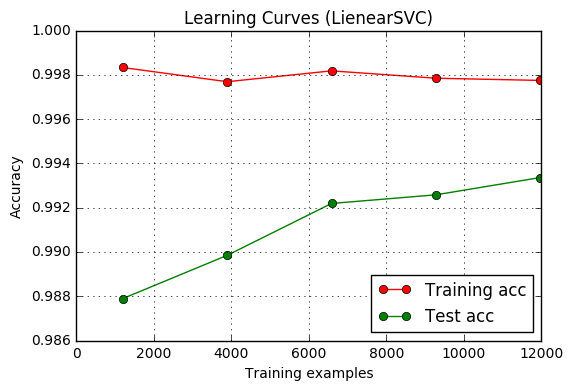
To know if is could be useful to add more training data, I make the learning curves:

The code to make this is after the cell in the main.ipynb titled "Plotting the learning curves to get some intuition of the classifier". This plot shows that adding more training data may help. So, I decided to train the classifier using both the train and the test data. The code for that can be found after the cell in the main.ipynb "Training the classifier with the optimal value of C with all the samples".

Sliding Window Search

A descrption of how (and identify where in my code) I implemented a sliding window search. How did I decide what scales to search and how much to overlap windows?

I made two version of a sliding window. One inefficient that take features of each window and another one that takes advantage of taken the HOG features of the hole image and the sliding window. The main code of this two version is taken from the lessons of this nanodegree.

The ineficiente is split into two function; the first one, slide_window() in my_lesson_functions.py, return the coordinates of each window; the second one, search_windows() in my_lesson_functions.py,recive the coordinates of each window and classify it to return only the windows where a vehicles is posible to be. It's woth to note that in the original slide_window() I found an error in the compute the number of windows in x/y:

Before:

nx_windows = np.int(xspan/nx_pix_per_step) - 1
ny_windows = np.int(yspan/ny_pix_per_step) - 1

Now:

nx_windows = np.int((xspan - xy_window[0])/nx_pix_per_step) + 1
ny_windows = np.int((yspan - xy_window[1])/ny_pix_per_step) + 1

The another one, find_cars(), extract features of the whole image using hog sub-sampling and make predictions. Although is more inefficient, I find more convenient to modify the original function in order to return the coordinates of the predicted windows instead of the image with the detected window. Similar as before, I find an error in original function:

Before:

nxsteps = (nxblocks - nblocks_per_window) // cells_per_step 
nysteps = (nyblocks - nblocks_per_window) // cells_per_step

Now:

nxsteps = (nxblocks - nblocks_per_window) // cells_per_step + 1
nysteps = (nyblocks - nblocks_per_window) // cells_per_step + 1

To decided the size of the windows and the percentage of overlapping between them, as well as where to begin and when to stop, I took the following consideration:

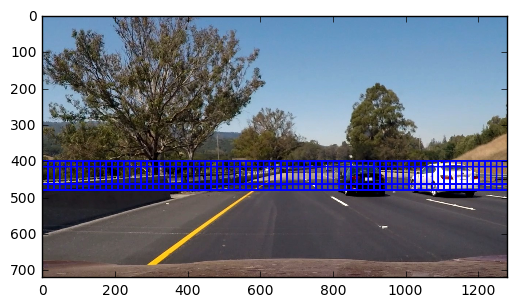
As is not reasonable to search a vehicle in the sky or in the trees, I choose that all the windows start near of the horizon. Visualizing a frame of a video I realize that the horizon is around the 400 row of the image frame.
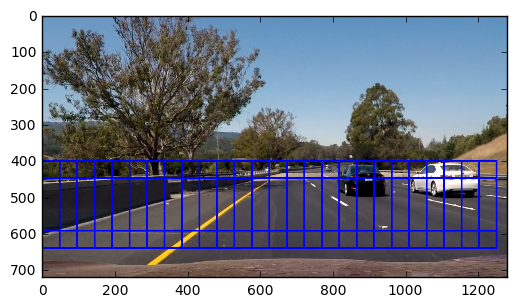
I notice that the window is not necessary to fit perfect to a car. The SVM is robust enough to predict vehicle even when the car is partially in the image or are some noise around the car. So, in order to keep low the number of windows search, I decide to use only three sizes: 64, 128 and 192. But to have a more precise localization of the vehicle I decide to have high overlapping, an overlapping of 75%.
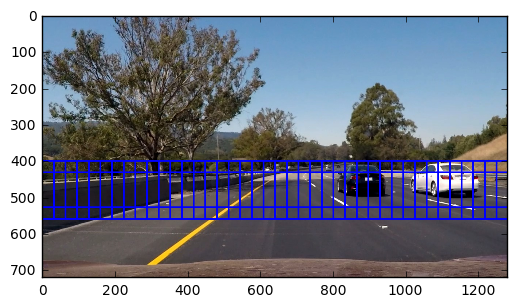
I choose to stop y variable to have two vertical windows of each scale.

Here I show the examples of each window scale

The 64 window size:

The 128 window size:

The 192 window size:

As the execution time with this setting was much less with features of the whole image using hog sub-sampling (0.6 seconds) than the features for each window (2 seconds) I decided to use the hog sub-sampling method.

Some examples of test images

Some examples of test images to demonstrate how my pipeline is working. What did I do to optimize the performance of my classifier?

As the performance of the classifier is good enough (99.33 % of accuracy) and I test that if a manually select a window the classifier predict most of the time right, I conclude that the parameters of the multiscale sliding window have a big influence in the result, that's why I play with only that parameters not with the classifier.

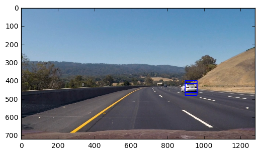
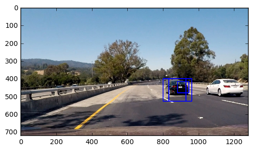
Here I show some examples of the test images:

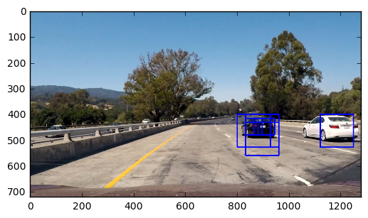
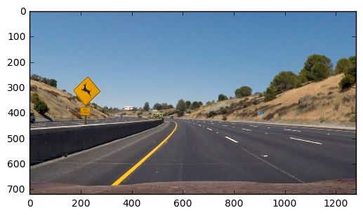
Ultimately I searched on two scales using YCrCb 3-channel HOG features plus spatially binned color and histograms of color in the feature vector, which provided a nice result. Here are some example images:

On test1 On test2 On test3 On test4

A link to my final video output.

Filter for false positives and a method for combining overlapping bounding boxes

Description of how (and identify where in my code) I implemented some kind of filter for false positives and some method for combining overlapping bounding boxes.

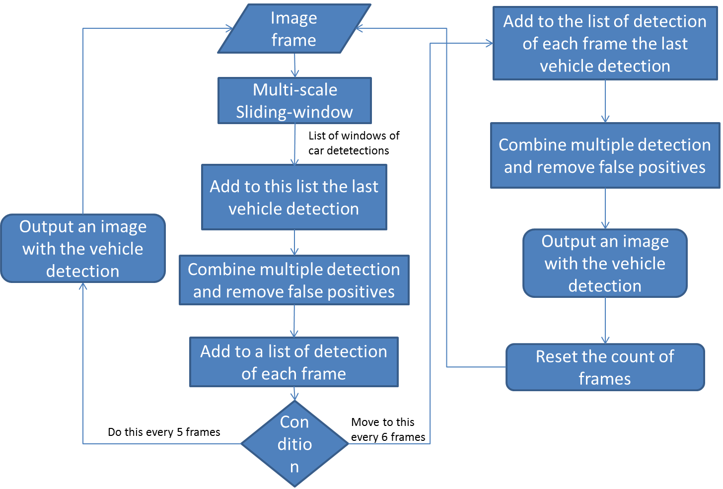
The complete pipeline can be found on the cells after the markdown cell titled "Let's make it in a video" in the notebook main.ipynb. To explain what I did I made the following diagram:

After applying the multiscale sliding window to one frame, I add to this detection list the last windows boxes output on the video (at the begin of the video is initialized with zero). Then apply a filter for false positives and a method for combining overlapping bounding boxes in the same way as the lesson in this nanodegree. I set the threshold to one because as I take into account the last detection boxes, If at least one new detection on the same area that the last one was found, is a good indicator that is the same object. This is done for 5 frames and in each one, the detections were stored in a list. When the 6th frame come, I add two times last vehicle detection and apply the same filter and method to mitigate the false positives and combine the multiple detections. The benefit of adding two times last vehicle detection is that eliminated more false-positives when retaining the true positives. The threshold this section was set to 2.

Discussion

A brief discussion of any problems / issues I faced in my implementation of this project. Where will my pipeline likely fail? What could you do to make it more robust?

The first problem that I faced was that I didn't notice the errors in computing the number of windows in both sliding windows implementations. The second one was that in the original hog sub-sampling method to do sliding window method has a line to change the dtype of the image. That add me a lot of noise. Because the feature vector obtained is very different if I use the original uint8 and in consequence, the predictions of the SVM are wrong. Was until I apply sliding window on a small image of 64 by 64 pixels in a way that has only one window, that I notice that difference. When I fixed, the results of my pipeline improve a lot. Another important choose of this project was in deciding the size of the windows in the sliding window. That has a big influence in the result.

My pipeline fails sometimes, detecting the vehicles that drive in the opposite direction (I considering that as false positives). Another problem is that sometimes detect two cars where is only one car. Although that was for a very short period of time may be this can be solved make it more robust.

To make it more robust I think that adding more training example doesn't help too much, but adding more training classes may be useful. For example, we can train the follower classifiers:

One to predict if an object in an image is a left-car or not-left-car (not-left-car can be car too but in other orientation).
Other to predict if an object in an image is a right-car or not-right-car (not-right-car can be car too but in other orientation).
Other to predict if an object in an image is a middle-car or not-middle-car (not-middle-car can be car too but in other orientation).

With that, we can search in sliding window method only on the sides of the road that is more likely to find a car with that orientation.

Independently of this, train a classifier that output a probability instead of only the class may help a lot. The reason is that we can code a filter to reduce false positives and combine overlapping windows base on this probabilities, not in the class. A neural net or a logistic regression are good candidates to do that job.

jjaviergalvez/CarND-Vehicle-Detection