Discrete densities

A python3 module to work with discrete (mostly integer valued) densities.

Dependencies:

Python3
ast, re, op
Used for some basic parsing expressions (not crucial)
op, heapq, functools.reduce, itertools.product
Used for MultiDensity
math
Used for gaussMap and stdev
matplotlib
Used for graphical plotting (plot_image, plotImage)
median
Used for median
functools.lru_cache, functools.wraps Used for memoized_method (performance related, could be removed)

Files:

densities.py
Main content
- Defines the following classes:
  - Density
  - Die
  - Constant
  - Zero
  - One
  - MultiDensity
- Defines the following functions:
  - get_plot
  - get_simple_plot
  - plot_image
  - AdvantageDie
  - DisadvantageDie
  - DieExpr
combatant.py Combatant module for combat simulations, see COMBATANT.md.
main.py
Examples on how to use/apply densities.py
test.py
A simple example for simulating combats between DndNealTestCombatant.

Documentation:

Density

The module works with discrete distributions (e.g. die rolls). The main class used everywhere is "Density" which refers to the probability mass function. See https://en.wikipedia.org/wiki/Probability_mass_function for more information. Basically a "Density" encodes all possible outcomes of a (discrete) random variable together with their probability.

Let's take the example of a d20 die roll which is a (discrete) random variable with 20 possible outcomes all with probability 1/20. These possible outcomes together with their probability are all stored in the density class Die(20).

⚠️
For all operations/methods defined below we assume that the corresponding random variables are independent.

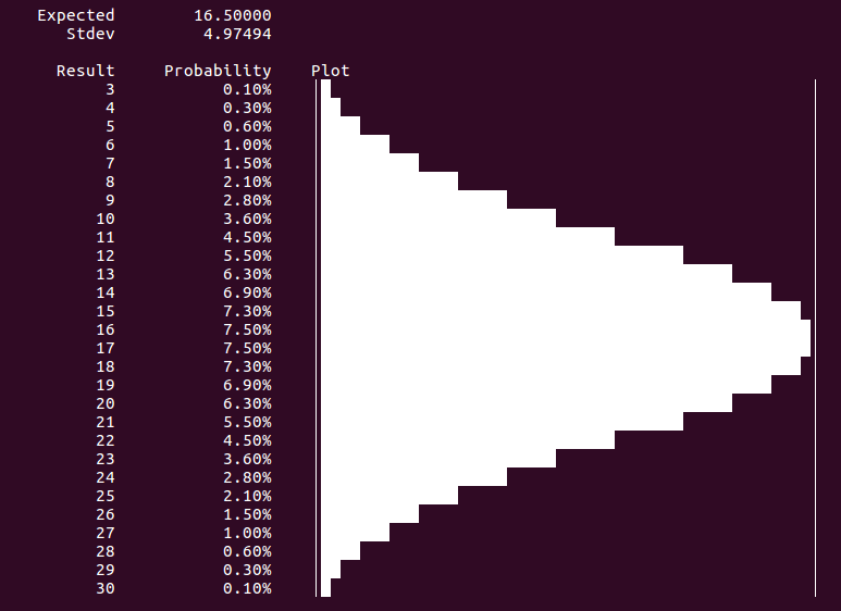
The standard string representation of a density (use print(density)) lists all outcomes together with their probabilities and also gives a (text) plot of the probability mass function. In addition also the expected value and the standard deviation is displayed.

Screenshots

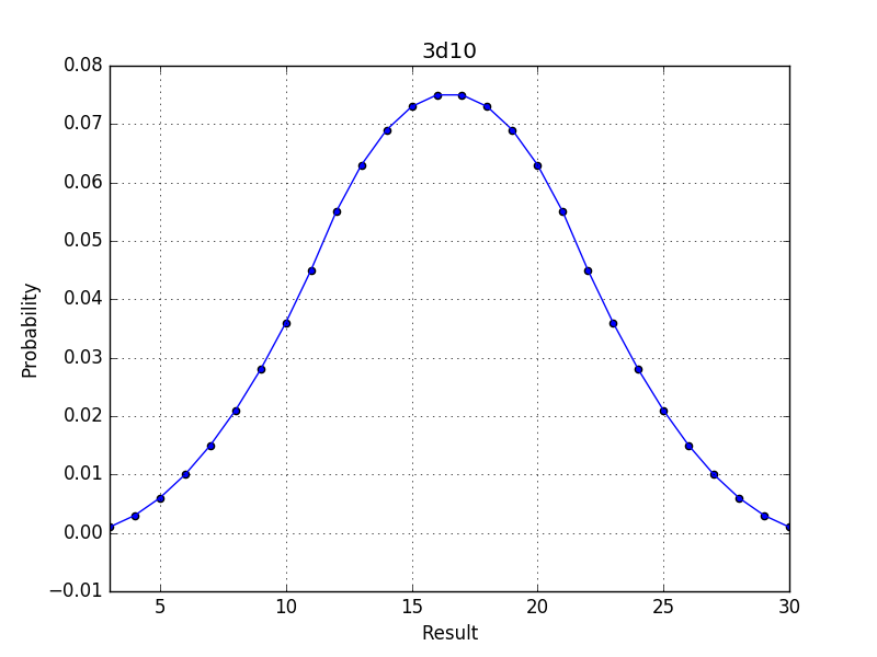
    print(d10+d10+d10)

    (d10+d10+d10).plotImage("3d10")

Defining densities

A density can be directly specified by passing it a dictionary of all (key,probability) entries. For example the following would directly define a d20 die roll density:

    densityDict = {}
    for r in range(1, 20):
      densityDict[r] = 1.0 / 20
    d20 = Density(densityDict)

However there are already predefined classes for this:

Die(n)
A die with n sides, i.e. n possible outcomes all with probability 1/n
Constant(n)
A constant density, i.e. 1 possibly outcome (n) with probability 1
Zero
The constant density for n=0
One
The constant density for n=1
AdvantageDie(n)
The density corresponding to rolling two Die(n) and taking the larger result.
DisadvantageDie(n)
The density corresponding to rolling two Die(n) and taking the smaller result.
MultiDensity(...)
Used to define more complex densities built from multiple other densities (see below for more details).

To simplify expressions it is recommended to define abbreviations for commonly used densities:

    d2   = Die(2)
    d3   = Die(3)
    d4   = Die(4)
    d6   = Die(6)
    d8   = Die(8)
    d10  = Die(10)
    d12  = Die(12)
    d20  = Die(20)
    d100 = Die(100)
    ad20 = AdvantageDie(20)
    dd20 = DisadvantageDie(20)

Binary operations between densities

Addition and Subtraction
D1 + D2 is the density corresponding to adding the two corresponding random variables. Mathematically speaking the addition of densities forms a commutative monoid with identity Zero. For example d20+d20 is the density of two added d20 rolls with possible outcomes ranging from 2 to 40.

Example:
```
  print(d6 + d4)
  print(d6 - d10)
```
Multiplication
D1 * D2 is the density corresponding to multiplying the two corresponding random variables. Mathematically speaking the multiplication of densities forms a commutative monoid with identity One. For example d2*d20 is the density corresponding to rolling a d2 and d20 and then multiplying the two results.

Example:
```
  print(d3*d6)
```
Integers and floats
In place of a density one can also use regular integers and/or floats in operations. In this case the integer/float is considered a Constant density. Mathematically speaking multiplication by integers is distributive with respect to addition. For instance d20 + 10 is the same as d20 + Constant(10), i.e. the density corresponding to rolling a d20 and adding 10 with outcomes ranging from 11 to 30 (with probabilities 1/20).

⚠️
This can be particularly confusing with multiplication: 2*d20 is the same as Constant(2)*d20 and not the same as d20+d20. Constant(2)*d20 corresponds to rolling a d20 and multiplying the result by 2 with outcomes 2, 4, ..., 40 (with probabilities 1/20). Adding the same density n times can be achieved with the method arithMult (see below). E.g. d20 + d20 + d20 is the same as d20.arithMult(3)

Example:
```
  print(3*d6)
  print(d6 + d6 + d6)
  print(d6.arithMult(3))
```
More general binary operations
An arbitrary binary operations between two densities can be defined using the method D1.binOp(D2, operation) where operation is a function in two variables operation(outcome1, outcome2) that defines the final outcome in case the outcome of D1 is outcome1 and the outcome of D2 is outcome2.

For example d20.binOp(d4, lambda a, b: a+b) gives the same as d20 + d4 and d20.binOp(d20, lambda a,b: max(a,b)) gives the same as d20.with_advantage().

(Unary) operations on densities

The following methods are defined on a given density d:

d.arithMult(n)
Gives the density d + ... + d (n times) in case n is a nonnegative integer. Mathematically speaking arithmetical multiplication by integers is distributive with respect to addition of densities. It is also possible use a density secondDensity with nonnegative integer outcomes as an argument. In this case the resulting density corresponds to first rolling secondDensity and then rolling that many d. In this case the arithmetical multiplication is no longer distributive.

Example:
```
  print(d20.arithMult(3))
  print(d20.arithMult(d4))
```
-d
Gives the density d with outcomes of opposite sign
abs(d)
Gives the density d with outcomes replaced by their absolute value
d.conditionalDensity(condition)
Gives the density d but only with outcomes that satisfy the given condition. Note that this increases the probability of the remaining outcomes.

For example d20.conditionalDensity(lambda a: a<=6) is the same as d6.
d.with_advantage()
Returns the density d corresponding to taking an outcome from d twice and dropping the lower outcome.

⚠️
Note that densities in general don't keep track of how they were created. E.g. (d20 + d6 + d4).with_advantage() does not correspond to rolling a d20, d6, d4 and dropping the lowest. Instead it corresponds to rolling and adding all three twice and then dropping the lower result of that, giving a density with outcomes ranging from 3 to 30. See the section regarding MultiDensity in case you want to define operations on multiple densities.
d.with_disadvantage()
Returns the density d corresponding to taking an outcome from d twice and dropping the higher outcome.
d.summedDensity(n)
Let's say we add d arbitrary often to itself and then we check how many times (k) we had to do the addition to reach at least n. d.summedDensity(n) returns the density / probability mass function for k.

For example let's say it takes d6+d6 minutes to find 1 food portion. If we keep searching one might ask: How much food can I expect after searching one hour? The corresponding density / distribution in this case can be found by (d6+d6).summedDensity(60) (with expected value (d6+d6).summedDensity(60).expected()). Here is an example on how to plot the expected number of food portion in terms of how long you search (both as text plot and as image plot):
```
  twod6 = d6+d6
  def expectedFood(minutes):
    return twod6.summedDensity(minutes).expected()
  get_plot(expectedFood, range(0, 100+1))
  plot_image(expectedFood, range(0, 100+1))
```
d.roll()
Returns a randomly selected outcome of the density (according to the distribution). Again the density does not keep track of how it was created only one final result will be returned.

Example:
```
  print((d10+d6).roll())
  print((d10+d6).roll())
```
d.asMultiDensity(n)
Returns a MultiDensity involving n copies of the given density (i.e. MultiDensity(d, ..., d) where d occurs n times). See the section on MultiDensity for further information...
d.plot()
Returns a text representation of the density d. This is implicitly called when doing print(d).
d.plotImage(name="plot")
Stores an image representation of the density in a file (default name: "plot.png"). See the section regarding plotting for more information...
d[n]
Returns the probability for the outcome n
d.keys(), d.values()
Returns the (sorted) possible outcomes resp. the corresponding probabilities
d.isValid()
Returns if d is a valid density (i.e. that the probabilities of all outcomes really add up to 1.0).
d.expected()
Returns the expected value of the density
d.variation()
Returns the variation of the density
d.stdev()
Returns the standard deviation of the density
d.cdf
Is the cumulative distribution function of the density. I.e. d.cdf(n) gives the probability that d<=n.
d.inverseCdf
Is the inverse cumulative distribution function of the density. I.e. d.inverseCdf(p) returns the smallest outcome n such that d.cdf(n)>=p.
d.median()
Returns the median of the density
d.normalApproximation
Is the (continuous) Gauss map with the same standard deviation and expected value as the given density
d.isZero() Returns if d is the Zero density
More general unary operations
An arbitrary unary operation on the given density can be defined using the method d.op(operation) where operation is a function in one variable operation(outcome) that defines the final outcome in case the outcome of d is outcome.

For example d20.op(lambda a: max(a)) gives the same as max(d20).

Probability calculations

For densities the usual comparison and equality operators don't return Boolean results. Instead they return the probability for the given condition. For example:

Comparison and Equality operators
The usual comparison operators can be used: <, <=, >, >= The equality operators can be used: ==, != The following returns the probability that (d6+d10) is smaller or equal to d8 (including a nice way to print the result as a probability):
```
  d6+d10 <= d8
  print("{:.4%}".format(d6+d10 <= d8))
```

⚠️
As already described in the sections "Integers and floats" one can also be used in the condition which are then treated as constant densities. For example d10 > 7 gives the probability that a d10 roll is larger than 7.

More general conditions for calculating probabilities The probability of an arbitrary condition on the density can be calculated using the method d.prob(condition) where condition(outcome) is predicate function (i.e. it returns whether the corresponding outcome should be included or not), d.prob(condition) then returns the probability that the given condition is satisfied.

Example:
```
  d20.prob(lambda a: a!=6 and a<14)
```

Density calculations involving multiple densities

The class MultiDensity can be used to do/define operations on multiple densities. To generate a MultiDensity a list of densities have to be passed.

Example:

    threeD20 = MultiDensity(d20, d20, d20)

The MultiDensity itself is also a density corresponding to the addition of the given densities (in this example d20 + d20 + d20) and all operations and methods of regular densities can be done on MultiDensity (they don't take into account the individual densities though, just the final sum).

⚠️
Note that MultiDensity(d2,d6).drop_lowest() (and similarly for the other methods) is not the same as MultiDensity(d2,d6).with_advantage(). The first case corresponds to rolling a d2 and a d6 and then dropping the lower result of the two. The second case corresponds to rolling d2+d6 twice and then dropping the lower result of the two. In the first case the outcomes range from 1 to 6, in the second case the outcomes range from 2 to 8.

In addition the following (multi density) methods can be used:

d.drop_highest(n=1)
Returns a (regular) density corresponding to rolling all defined individual densities and then dropping the highest n rolls of those (default: n=1).

Example:
```
  multiDensity = MultiDensity(d2, d6, d20)
  print(multiDensity.drop_highest(2))
```
d.drop_lowest(n=1)
Returns a (regular) density corresponding to rolling all defined individual densities and then dropping the lowest n rolls of those (default: n=1).

Example:
```
  multiDensity = MultiDensity(d2, d6, d20)
  print(multiDensity.drop_lowest())
```
d.keep_highest(n=1)
Returns a (regular) density corresponding to rolling all defined individual densities but only keeping the highest n rolls of those (default: n=1).

Example:
```
  multiDensity = MultiDensity(d2, d6, d20)
  print(multiDensity.keep_highest())
```
d.keep_lowest(n=1)
Returns a (regular) density corresponding to rolling all defined individual densities but only keeping the lowest n rolls of those (default: n=1).

Example:
```
  multiDensity = MultiDensity(d2, d6, d20)
  print(multiDensity.keep_lowest(2))
```
d.combine(p1, ..., pn)
Returns a (regular) density corresponding to rolling all defined individual densities and picking one of them according to the probabilities specified.

Example:
```
  multiDensity = MultiDensity(d2, d6, d20)
  print(multiDensity.combine(1.0/3, 2.0/6, 2.0/6))
```
d.keepRandom()
Returns a (regular) density corresponding to rolling all defined individual densities and picking one of them at random. I.e. d.combine(1.0/n, ..., 1.0/n).

Example:
```
  multiDensity = MultiDensity(d2, d6, d20)
  print(multiDensity.keepRandom())
```
More general multi density operations
More general multi density operations can be defined using the method multiDensity.multiOp(operation) where operation is a function in as many variables as defined individual densities. operation(a1, ..., an) specifies the desired final outcome in case the outcome of the individual densities d1, ..., dn is a1, ..., an. The final result is a normal (non-multi) density (with the operation applied on the outcome combinations).

⚠️
Operations on many densities get slow quite fast.

Example:
```
  MultiDensity(d3, d6, d20).multiOp(lambda a,b,c: max(a,b,c)-min(a,b,c))
```

More examples
Sometimes one is interested in comparing two rolls in a complicated fashion. Let's say we compare two rolls and the following function determines the winner of the two rolls (1 meaning the attacker/first roll wins and 0 the defender/second roll):

  bonusAttacker = 10
  bonusDefender = 0
  def successCondition(attackRoll, defendRoll):
    if (defendRoll == 20):
      return 0
    if (defendRoll == 1):
      return 1
    if (attackRoll + bonusAttacker > defendRoll + bonusDefender):
      return 1
    else:
      return 0

We can get the distribution who's winning (i.e. when successCondition is 1 resp. 0) as follows:

  attackerDie = ad20
  defenderDie = d20
  successDensity = MultiDensity(attackerDie, defenderDie).multiOp(successCondition)

Of course this could be generalized to more rolls... Since in this case only two rolls are involved this could also be written as attackerDie.binOp(defenderDie, successCondition).

To get the probability that the attacker wins we can simply do:

  successDensity > 0

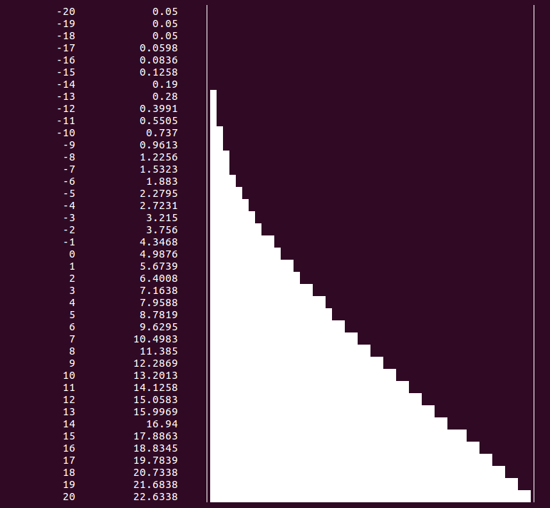
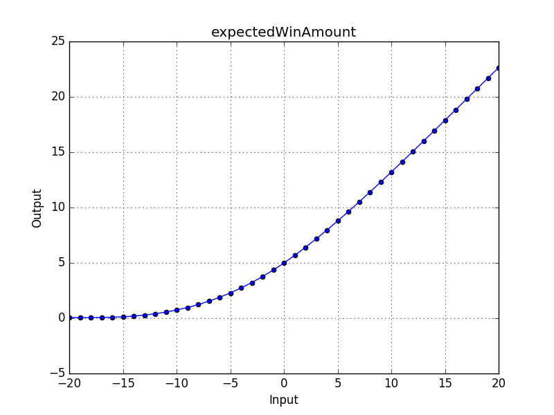
But maybe we want to know the success probability for different values of bonusAttacker, not just bonusAttacker = 10 and maybe we don't just want the success probability but also some kind of measure by how much the attacker won. Let's say we want to know the expected amount by which the attacker wins, parametrized by bonusAttacker (always assuming bonusDefender=0) in some range. We can do this by first parametrizing the winAmount condition (by bonusAttacker resp. bonusDefender):

  attackerDie = ad20
  defenderDie = d20
  def winAmount(bonusAttacker, bonusDefender):
    def finalAmount(attackRoll, defendRoll):
      if (defendRoll == 20):
        return 0
      if (defendRoll == 1):
        return max(1, (attackRoll + bonusAttacker) - (defendRoll + bonusDefender))
      if (attackRoll + bonusAttacker > defendRoll + bonusDefender):
        return (attackRoll + bonusAttacker) - (defendRoll + bonusDefender)
      else:
        return 0
  def expectedWinAmount(bonusAttacker):
    bonusDefender = 0
    winAmountDensity = MultiDensity(attackerDie, defenderDie).multiOp(winAmount(bonusAttacker, bonusDefender))
    return winAmountDensity.expected()
  get_plot(expectedWinAmount, range(-20,20))
  plot_image(expectedWinAmount, range(-20,20))

Note that expectedWinAmount is not a density, it's just a function but there are also some generic plotting methods for functions: get_plot for text plots and plot_image for image plots (see the section on Plotting for more information).

Plotting

There are some helper plotting functions defined that are being used:

Text plotting
```
get_plot(p, inputs=range(-20, 20+1), plotWidth=50, minP=None, maxP=None, asPercentage=False, centered=True)
```
- p
  The function to plot, e.g. expectedWinAmount
- inputs
  The function inputs, default: range(-20, 20 + 1)
- plotWidth
  The desired plot width, default: 50
- minP, maxP
  The desired plotting range. If unspecified minP is set to the smallest result if that's below zero and to zero if no result is below zero. If unspecified maxP is set to the maximal result (for probabilities it might make sense to set maxP=1.0).
- asPercentage
  Determines if the results are shown as percentages, default: False
- centered
  Determines if negative results are drawn away from the zero line or if everything is always drawn from the left up to the value, default: True (away from zero)
If the default values are fine a simple get_plot(function) can be used. If only the second column is desired (e.g. to easily copy the results), use get_simple_plot in place of get_plot.

Example (see above for the definition of expectedWinAmount or use a different function):
```
  print(get_plot(expectedWinAmount))
  print(get_simple_plot(expectedWinAmount))
  print(get_plot(expectedWinAmount, range(-20, 20 + 1), plotWidth = 50, minP = 0.0, maxP = 1.0, centered = True, asPercentage = True))
```
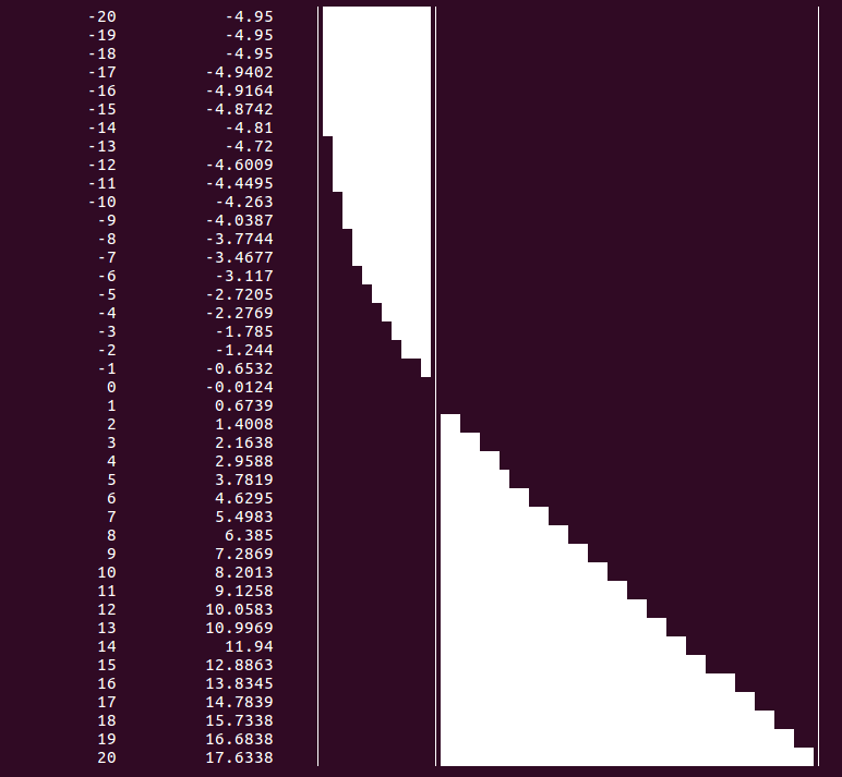
Also plotting of negative values is possible. In this case a line indicating zero is drawn:
```
  print(get_plot(lambda k: expectedWinAmount(k) - 4))
```
Image plotting
For image plotting the following function can be used:
```
plot_image(function, inputs=range(-20, 20+1), name=None, xlabel="Input", ylabel="Output", fmt='-', **kwargs)
```
If name is not specified then the function name is used if possible, if that's not possible then plot is used. The function will save the image plot in the file given by the name (as a .png file). The function uses matplotlib. For possible plotting formats, other additional arguments or in general more complex plotting see:

https://matplotlib.org/api/_as_gen/matplotlib.pyplot.plot.html#matplotlib.pyplot.plot

Example:
```
  plot_image(expectedWinAmount)
```
Text plotting of densities
For densities the method plot(plotWidth=70) can be used which internally calls get_plot. Or even more simply print(density) can be used...

Example:
```
  (d20+d20+d20).plot(90)
  print(d20+d20+d20)
```
Image plotting of densities
For densities the method plotImage(name="plot") can be used which internally calls plot_image.

Example:
```
  (d20+d20+d20).plotImage("3d20")
```

More advanced plotting
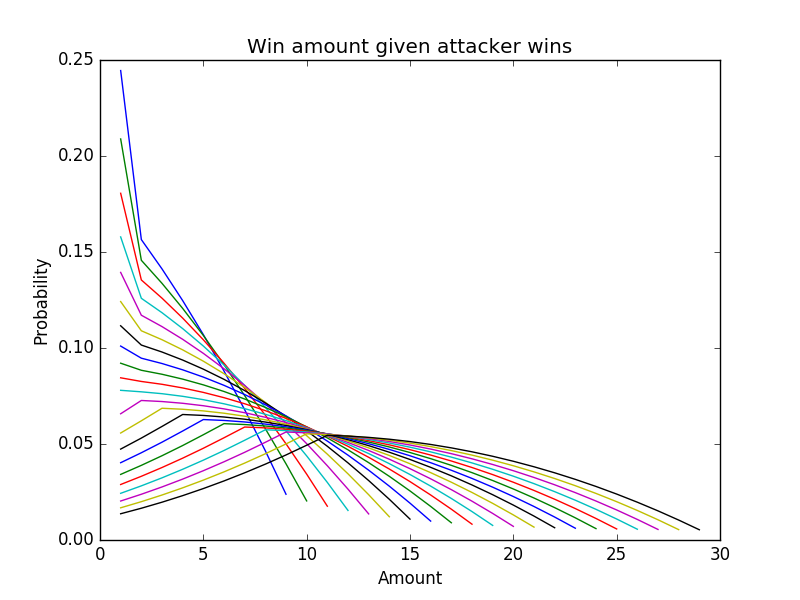
For more complex plotting, pyplot should be used directly, example:

  fig = plt.figure()
  plt.title("Win amount given attacker wins")
  plt.xlabel("Amount")
  plt.ylabel("Probability")
  for bonusAttacker in range(-10,10+1):
    d = expectedWinAmount(bonusAttacker).conditionalDensity(lambda k: k>0)
    plt.plot(d.keys(), d.values(), '-')
  plt.savefig("winAmountAttackerWins")
  plt.close(fig)

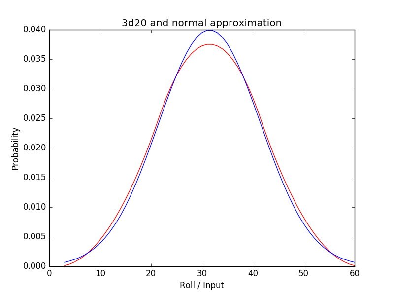
Here is another example that plots d20+d20+d20 and it's normal approximation:

  fig = plt.figure()
  plt.title("3d20 and normal approximation")
  plt.xlabel("Roll / Input")
  plt.ylabel("Probability")
  m3d20 = d20 + d20 + d20
  plt.plot(m3d20.keys(), m3d20.values(), '-r')
  normalApproximation = m3d20.normalApproximation
  plt.plot(m3d20.keys(), [normalApproximation(k) for k in m3d20.keys()], '-b')
  plt.savefig("3d20vsNormal")
  plt.close(fig)

jjermann/dicedensity