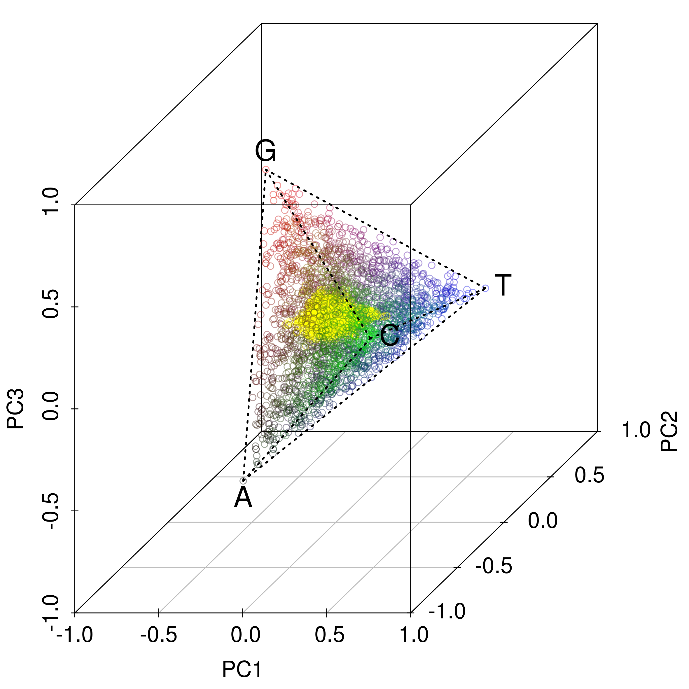
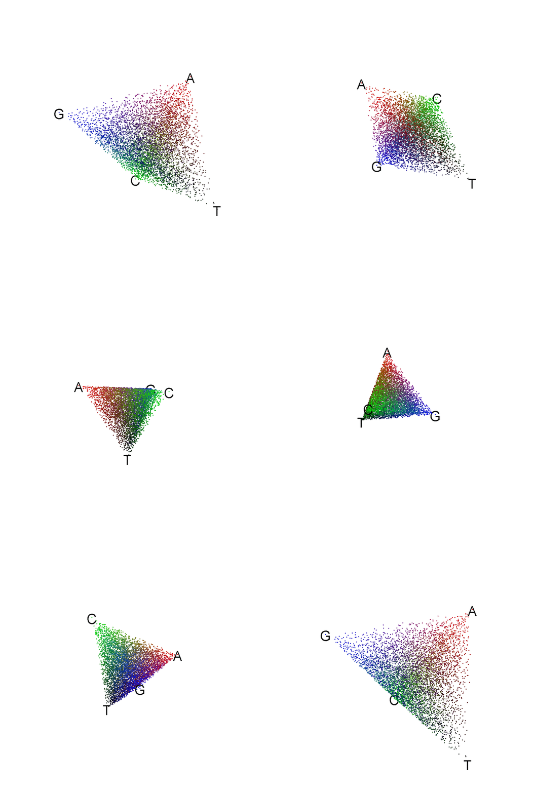
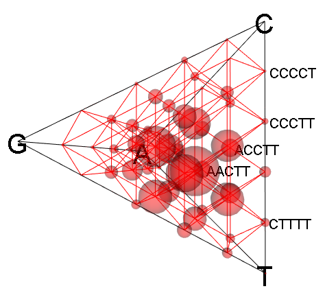
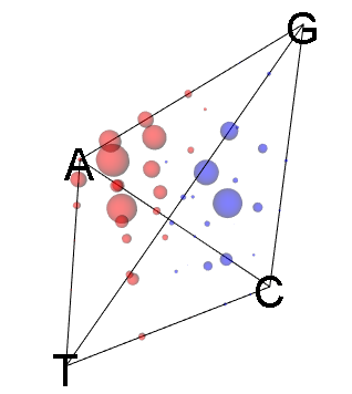
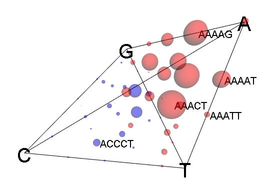
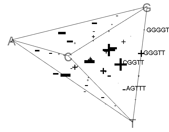
R package to visualize the acgt or k-mer distribution between samples.
source("http://bioconductor.org/biocLite.R")
biocLite("ShortRead")
Get the released version from CRAN:
## not available yet
## install.packages("kmerPyramid")
Or the development version from github:
# install.packages("devtools")
devtools::install_github("jkruppa/kmerPyramid")library(kmerPyramid)
data(viralExampleSeqs)
kmer_distr <- get_kmer_distribution(viralExampleSeqs, k = 1)
pyramid_3d(kmer_distr,
cex = 2,
color = "blue")
ids <- names(viralExampleSeqs)
pyramid_3d(kmer_distr,
ids = ids,
cex = 2,
color = "blue",
identify = TRUE)
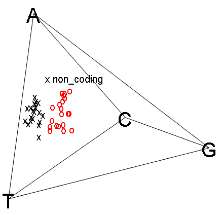
data(viralExampleCodingSeq)
kmer_distr <- get_kmer_distribution(viralExampleCodingSeq, k = 1)
text_ids <- ifelse(names(viralExampleCodingSeq) == "non_coding", "x", "o")
color_ids <- ifelse(names(viralExampleCodingSeq) == "non_coding", "black", "red")
pyramid_3d(kmer_distr,
cex = 1,
text = text_ids,
color = color_ids)
ids <- names(viralExampleCodingSeq)
pyramid_3d(kmer_distr,
ids = ids,
cex = 1,
text = text_ids,
color = color_ids,
identify = TRUE)library(kmerPyramid)
data(viralExampleSeqs)
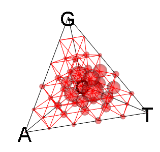
viral_window_list <- get_pca_window_list(viralExampleSeqs, window = 5)
pyramid_3d_grid(viral_window_list[1],
color = "red")pyramid_3d_grid(viral_window_list[1],
color = "red",
identify = TRUE)pyramid_3d_grid(viral_window_list[c(3,5)],
difference = TRUE)pyramid_3d_grid(viral_window_list[c(3,5)],
difference = TRUE,
identify = TRUE)pyramid_3d_grid(viral_window_list[c(3,5)],
difference = TRUE,
bw = TRUE,
bw.cex = 75,
identify = TRUE)This ia a R package. If you have never ever worked with R or a programing language, feel free to visit http://tryr.codeschool.com/ a free online school on R syntax and programing. This will give you a deeper insight than this tutorial is planed for.
The installation is very simple. Start R and copy and paste the following code. This will install devtools which is needed to install packages from this GitHub repository. In the next line the kmerPyramid package will be installed. This has only be done once, after installing use library(kmerPyramid) to load the package.
install.packages("devtools")
devtools::install_github("jkruppa/kmerPyramid")
We obtain a single random fasta file with three virus sequences under /data/virus.fa. This file can be directly loaded into R by using the package Biostrings. The package should be installed automatically by the kmerPyramid package. If not please follow the instructions under https://bioconductor.org/packages/release/bioc/html/Biostrings.html.
library(Biostrings)
sequence <- readDNAStringSet("https://raw.githubusercontent.com/jkruppa/kmerPyramid/master/data/virus.fa")
The following shows the three virus sequences in a DNAStringSet object. The sequences have different lengths and different ACGT contents. For a deeper understanding of the DNAStringSet objects please vists the site https://web.stanford.edu/class/bios221/labs/biostrings/lab_1_biostrings.html. To select single sequences use sequence[1] for the first sequence and names(sequence) to access the names.
R> sequence
  A DNAStringSet instance of length 3
    width seq                                               names
[1] 10000 CAAATTAAATTCTAAATGTTGAA...CTAGGTCTAATAAAGAATCATTA virus_1
[2]  8000 CCGCCCCGAGGCCGCGCGTGCTC...CGCCCCGCGCCCCGCGCGCCCGG virus_2
[3]  6000 GTAAAATGAGAAAAAAAAACCGA...GAGAGTCAGAAAAAAAGAGAAAC virus_3
It is also possible to read in own fasta files using the path to the single file in readDNAStringSet()
library(Biostrings)
sequence <- readDNAStringSet("C:/path/to/my/fasta/my_fasta_file.txt")
If you have two files and would like to merge them into one single DNAStringSet do the following and go on with sequence.
sequence_1 <- readDNAStringSet("C:/path/to/my/fasta/my_fasta_file_sequence_1.txt")
sequence_2 <- readDNAStringSet("C:/path/to/my/fasta/my_fasta_file_sequence_2.txt")

sequence <- c(sequence_1, sequence_2)
Now you can compare single sequences with each other.
Very often you might want to compare two sequences given their k-mer distribution. In the first step the sequences must be processed by the function get_pca_window_list(), where the k-mer disribution of the given window size is computed. As a rule of thumb, the differences between species start at the 5-mer distribution. Therefore, it might be feasible to use a window size of 5.
library(kmerPyramid)

## We produce the 5-mer distribution
viral_window_list <- get_pca_window_list(sequence, window = 5)

## We compare the sequence 1 to 2
pyramid_3d_grid(viral_window_list[c(1, 2)],
                difference = TRUE,
                identify = TRUE)
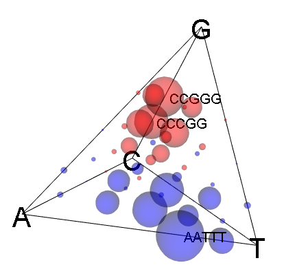
The following plot will be openend and can be moved by the mouse. The window might a little bit small, so pull it larger.
If you klick with the right mouse button on different bubbles you get the assigned k-mer. Like CCGGG, CCCGG, and AATTT in the example picture. It is always sequence 1 minus sequence 2. Blue means an increase and red means a decrease of the given k-mer.
