Authors: Jesse Markowitz, Dillon Medd, Ronak Parekh
Home buyers in King County, WA, must weigh several factors when purchasing a house, balancing budget, location, size, and ovearall quality. King County includes Seattle and is the most populous county in the state of Washington. However, it also contains large rural and mountainous areas to the east, stretching to the Cascade Range. This provides a lot of choice and variety to prospective bome buyers.
In this analysis, we seek to identify the most important factors that contribute to the price of a home so that home buyers in King County can set reasonable expectations and make informed assumptions about what they will find.
What features correlate most with price? How does distance from the Seattle city center affect the price per square foot of a house?
Analysis and modeling through regression yield the following factors as predictive of house prices in King County:
- Square footage of the house
- Grade based on King County grading system
- Distance from Seattle city center
Together, these factors account for 72% of the variance in home prices in the county.
We identify these features through exploratory data analysis using housing sales data from King County. This dataset includes the sale price and a variety of features for houses sold in the county from May 2014–May 2015.
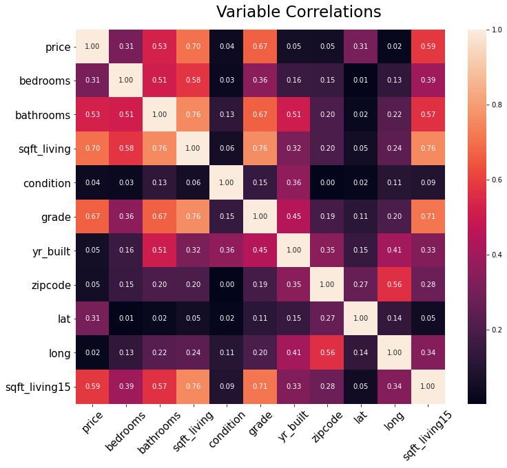
The correlation heatmap matrix below identifies sqft_living, grade, and sqft_living_15 as strongly correlated with price.
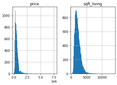
The distributions for price and sqft_living are heavily skewed right by outliers. Rather than drop these homes from the dataset, we instead log-transform these variables.
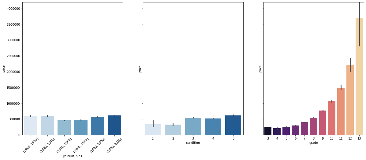
Factors like the age of a house (here given via yr_built) and the general condition are often major considerations for prospective home buyers. Let's compare these variables with grade, which denotes the construction quality, design, and adherance to building codes--a variable that (from the heatmap above) we already know correlates strongly with price.
Clearly, age (year built) has little impact on the price of a house. Condition does somewhat, although it's worth noting that very few houses are in the 1-2 range; the majority are in category 3. Grade has an enormouse impact (although very few houses are in the 12-13 range, which denotes high-quality, custom-built and -designed houses).
After noticing that many of the most expensive homes in the dataset had Seattle zip codes, we decided to investigate the relationship between distance from Seattle's city center and price of home.
Haversine Distance function returns distance (in kilometers) when given two locations longitude and latitude. Source
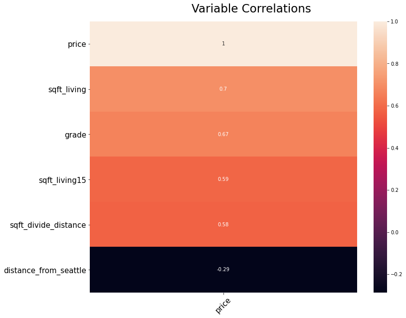
The Distance From City Center function returns a given location's distance from the center of Seattle. We use the function to create a new feature (column) in the DataFrame, then check the correlations with our new features.
As expected, distance_from_seattle has a negative correlation with price. The farther out from the city you are (higher distance), the lower the price overall tends to be (and the lower the price per square foot).
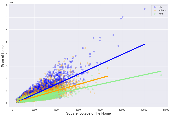
Now let's split the dataset into city, suburb, and rural homes. Using google maps we approximated the ranges for city (<12 km), suburb(12-25km), and rural (25+km) homes. If we run a series of simple linear regression with sqft_living as the only factor on price, disaggregated by location (city, suburb, and rural), we can evaluate the slope of each model. The slope represents price per square foot.
- Coefficient for city: 408.127
- Coefficient for suburb: 255.370
- Coefficient for rural: 192.927
This shows that the price per square foot is highest in the city, decreasing as the distance from the city center increases.
The visualization above shows the relationship between square footage of the house and price within the three different locations.
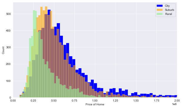
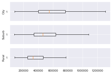
Here we take a look at the distribution of house prices within each location subset.
Now let's put it all together to create a model that predicts house prices for King County, WA.
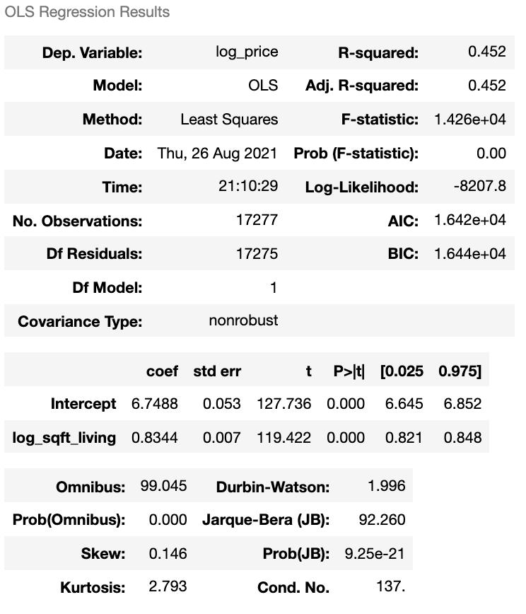
The simplest model is one that uses only size (sqft_living)) to predict the price (price)) of a house. We begin with this baseline for model validation, comparing this model to the model based on the features explored and engineered above.
The baseline model has an
- Baseline mse on training data: 0.1514145280654338
- Baseline mse on testing data: 0.14936244222233772
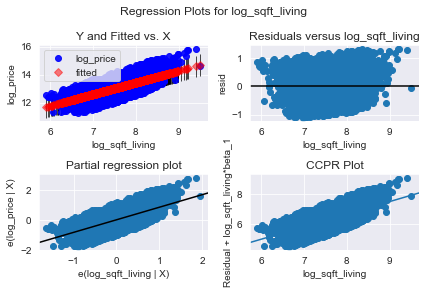
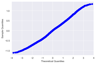
The Q-Q plot suggests our model and data adhere to assumptions of linearity. Our mse values are similar for both training and testing data, indicating our model is neither over nor under fit.
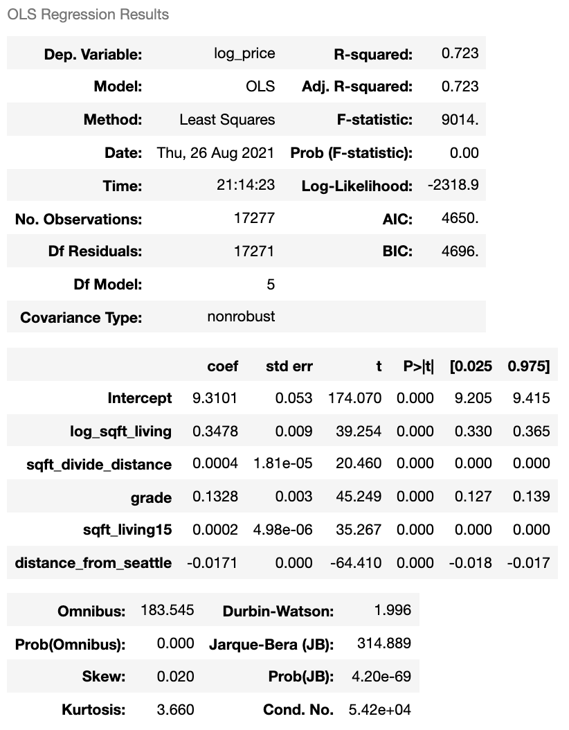
This model shows a great improvement over our baseline. The
Let's check residuals and mean square error again:
- Baseline mse on training data: 0.0765781972426975
- Baseline mse on testing data: 0.07597046311166614
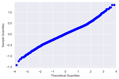
The Q-Q plot is still close to linearity. The mse values have improved dramatically--nearly cut in half from the baseline model. The similar scores between training and testing mse continue to suggest our model has consistent predictive power for seen and unseen data.
Our final model shows that price is affected most by square footage, grade, square footage of neighboring houses, and distance from Seattle city center. The model accounts for 72% of variance in housing prices (r2 = 0.723) and has consistent predictions for both training and unseen data.
- Price per square foot is largely predicted by distance from Seattle city center
- Higher in the city, lower farther out
- Buyers must balance optimal size and location for their budget
- Grade (structural quality) matters more than age or condition
Next steps:
- Compare recent sale price to original purchase price to determine trends and identify good areas for investment
- For a given budget, identify for buyers affordable house size (ft2) by location
- Use more detailed mapping to identify homes in urban, suburban, and rural areas.
See the full analysis in the Jupyter Notebook or review this presentation
├── Code
│   ├── Markowitz_working_nb.ipynb
│   ├── Ronak Notebook.ipynb
│   ├── Dillon Eda.ipynb
│   ├── Dillon_final_nb.ipynb
│
├── Data
├── Images
├── predicting_prices_king_county_jupyternb.ipynb
├── predicting_prices_king_county_presentation.pdf
└── README.md
