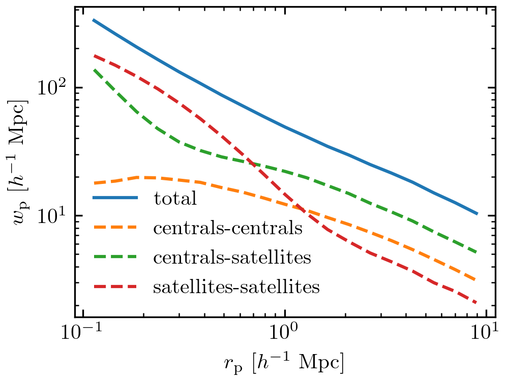
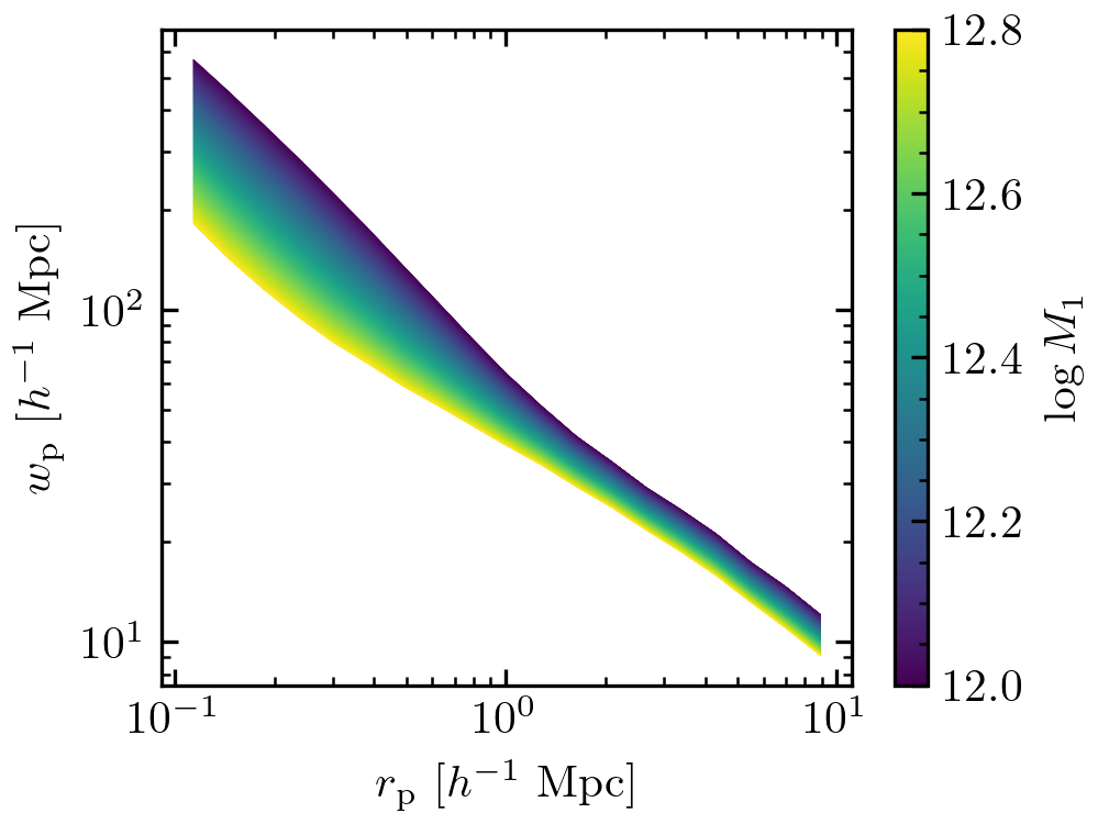
TabCorr: Tabulated Correlation Functions

This Python module provides extremely efficient and precise calculations of galaxy correlation functions in halotools using tabulated values. It is specifically intended for Markov chain monte carlo (MCMC) exploration of the galaxy-halo connection. It implements the method described in Zheng & Guo (2016) of tabulating correlation functions that only need to be convolved with the mean halo occupation to obtain the full correlation function of galaxies.

Installation

The package can be installed via pip.

pip install tabcorr

Usage

The following code demonstrates the basic usage of TabCorr.

import numpy as np
import matplotlib.pyplot as plt
import matplotlib as mpl
from halotools.empirical_models import PrebuiltHodModelFactory
from halotools.mock_observables import wp
from halotools.sim_manager import CachedHaloCatalog
from tabcorr import TabCorr

# First, we tabulate the correlation functions in the halo catalog. Note that
# by default, TabCorr applies redshift-space distortions (RSDs) in the
# tabulation of correlation functions.
rp_bins = np.logspace(-1, 1, 20)

halocat = CachedHaloCatalog(simname='bolplanck')
halotab = TabCorr.tabulate(halocat, wp, rp_bins, pi_max=40, verbose=True,
                           num_threads=4)

# We can save the result for later use.
halotab.write('bolplanck_wp.hdf5')

# We could read it in like this. Thus, we can skip the previous steps in the
# future.
halotab = TabCorr.read('bolplanck_wp.hdf5')

# Now, we're ready to calculate correlation functions for a specific model.
model = PrebuiltHodModelFactory('zheng07', threshold=-18)

rp_ave = 0.5 * (rp_bins[1:] + rp_bins[:-1])

ngal, wp = halotab.predict(model)
plt.plot(rp_ave, wp, label='total')

ngal, wp = halotab.predict(model, separate_gal_type=True)
for key in wp.keys():
    plt.plot(rp_ave, wp[key], label=key, ls='--')

plt.xscale('log')
plt.yscale('log')
plt.xlabel(r'$r_{\rm p} \ [h^{-1} \ \mathrm{Mpc}]$')
plt.ylabel(r'$w_{\rm p} \ [h^{-1} \ \mathrm{Mpc}]$')
plt.legend(loc='lower left', frameon=False)
plt.tight_layout(pad=0.3)
plt.savefig('wp_decomposition.png', dpi=300)
plt.close()

# Studying how the clustering predictions change as a function of galaxy-halo
# parameters is straightforward.
sm = mpl.cm.ScalarMappable(
    cmap=mpl.cm.viridis, norm=mpl.colors.Normalize(vmin=12.0, vmax=12.8))

for logm1 in np.linspace(12.0, 12.8, 1000):
    model.param_dict['logM1'] = logm1
    ngal, wp = halotab.predict(model)
    plt.plot(rp_ave, wp, color=sm.to_rgba(logm1), lw=0.1)

cb = plt.colorbar(sm, ax=plt.gca())
cb.set_label(r'$\log M_1$')
plt.xscale('log')
plt.yscale('log')
plt.xlabel(r'$r_{\rm p} \ [h^{-1} \ \mathrm{Mpc}]$')
plt.ylabel(r'$w_{\rm p} \ [h^{-1} \ \mathrm{Mpc}]$')
plt.tight_layout(pad=0.3)
plt.savefig('wp_vs_logm1.png', dpi=300)
plt.close()

Author

Johannes Ulf Lange

Citations

The method implemented in TabCorr has first been described in earlier work, particularly Neistein et al. (2011) and Zheng & Guo (2016). In Lange et al. (2019a), we developed a generalized framework for this method that also takes into account assembly bias. Finally, a good reference for the TabCorr code itself is Lange et al. (2019b).

License