This R-package has the purpose conveniently retrieving large geospatial point data stored on the cloud. It provides tools to select, filter, and download data of interest. Currently, only GEDI data is provided, but other sources, such as ICE-Sat2 may be added in the future.
You can install the development version of OpenEarthPoints with
devtools::install_github("joheisig/OpenEarthPoints")GEDI is a full-waveform LiDAR sensor with the mission of mapping biomass for global carbon dynamics research. The challenge with this data is its large volume. GEDI carries out several million measurements every day. These are processed to a table with close to 100 columns (Level 2A & 2B data), describing, e.g., elevation and canopy structure, which easily becomes larger than your computer’s memory. To handle such data we use (the R bindings of) cloud-compatible software tools Apache Arrow and Polars.
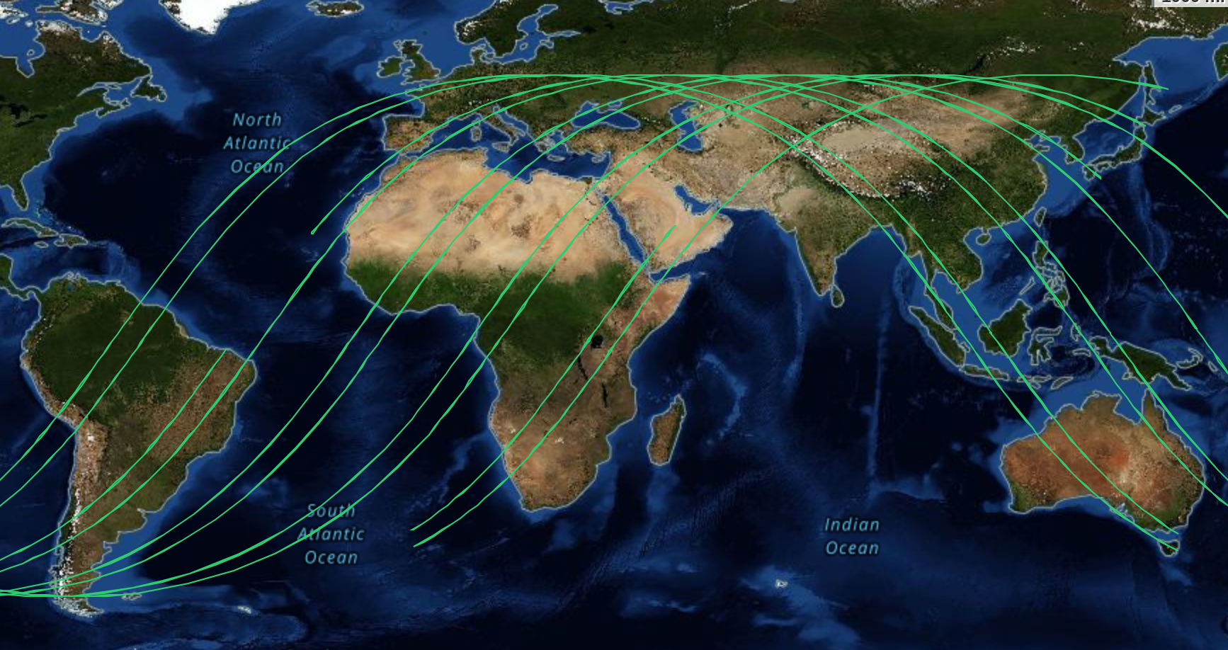
GEDI data is originally administered and distributed by NASA, yet not an easily accessible way. As GEDI in mounted on the ISS, it collects and stores data along its orbital flight path. However, data along a narrow line crossing all longitudes (on land and sea) is rarely useful in a spatial analysis.
Therefore, we pre-processed and re-chunked all available data from the start of the mission in April 2019 until the end of 2023 (with frequent updates planned). The dataset is stored on a Wasabi Simple Storage Service (S3) bucket, administered by OpenGeoHub and has ~5.4 billion observations (~1TB). It is organized as a partitioned Parquet dataset, which consists of one file per 5x5 degree tile and year. Parquet is a column-oriented file format with efficient storage and high compression properties.
library(OpenEarthPoints)
library(arrow)       # to handle parquet format
library(mapview) # interactive mapsThe best way to select GEDI data of interest is defining a place and a
time window. We can create a bounding box for spatial selection in
multiple ways. A convenient one is running the code below, which opens
an interactive map for drawing a bounding box by hand. To guide your
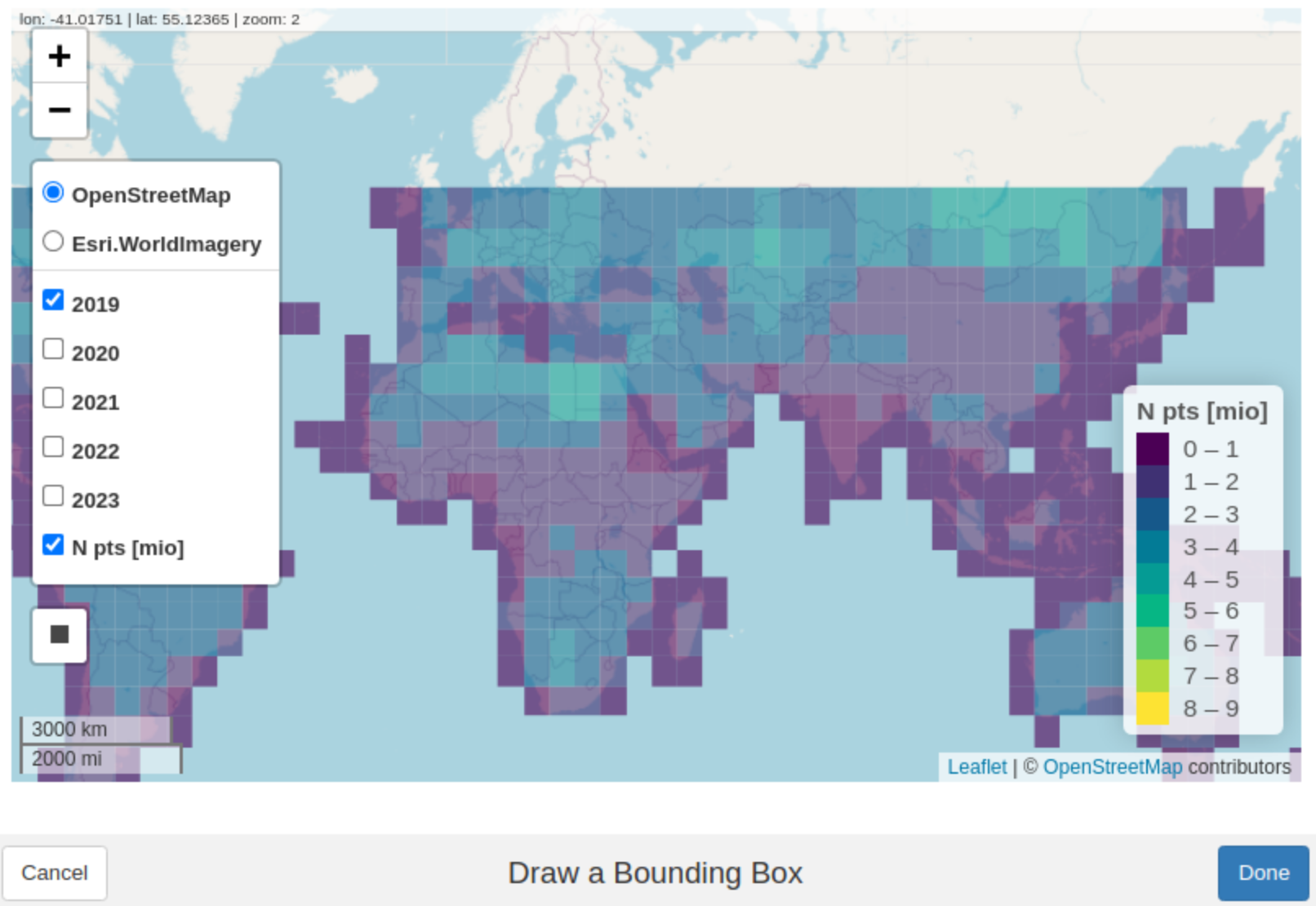
selection the interactive map shows all available 5x5 degree GEDI tiles
and their point counts (in millions) for each year The returned geometry
is stored in bb.
bb = draw_bbox()Let’s get an idea about the size of our bounding box:
sf::st_area(bb) |> units::set_units("km^2")
#> 144.4922 [km^2]If we are only interested in the data enclosed by the bounding box we
can pass it to our query and possibly add more selection and filter
options. Here you can specify a temporal selection (years) or a
selection of data columns (with options all, reduced, or a
character vector with desired column names). If you want to see all
available options, call show_gedi_columns().
Under the hood, bbox_query() uses the {polars} library to create (a
list of) optimized queries to the data on S3, which can be executed in
parallel.
q_bb = bbox_query(bb, years = 2020:2021, columns = "all")A {polars} query may look like this:
q_bb[[1]]$describe_optimized_plan()
#>
#>   Parquet SCAN https://s3.eu-central-1.wasabisys.com/gedi-ard/level2/l2v002.gedi_20190418_20230316_go_epsg.4326_v20240614/lon=0/lat=40/year=2021/gedi_l2_0.parquet
#>   PROJECT */94 COLUMNS
#> SELECTION: [(col("longitude").is_between([-0.096983, 0.088887])) & (col("latitude").is_between([44.189111, 44.27686]))]In case we want to study a larger area we can consider downloading
entire 5x5 degree tiles, which may be more efficient. Use tile_query()
with the bounding box from earlier and a selection of years to find
all intersecting tiles.
(q_tiles = tile_query(bb, years = 2020:2021))
#> Simple feature collection with 4 features and 5 fields
#> Geometry type: POLYGON
#> Dimension:     XY
#> Bounding box:  xmin: -5 ymin: 40 xmax: 5 ymax: 45
#> Geodetic CRS:  WGS 84
#> # A tibble: 4 × 6
#>     lon   lat  year dir                       n_points                  geometry
#> * <dbl> <dbl> <dbl> <chr>                        <int>             <POLYGON [°]>
#> 1     0    40  2021 /lon=0/lat=40/year=2021/…  2267680 ((0 40, 5 40, 5 45, 0 45…
#> 2     0    40  2020 /lon=0/lat=40/year=2020/…  3113049 ((0 40, 5 40, 5 45, 0 45…
#> 3    -5    40  2020 /lon=-5/lat=40/year=2020…  3058438 ((-5 40, 0 40, 0 45, -5 …
#> 4    -5    40  2021 /lon=-5/lat=40/year=2021…  2785341 ((-5 40, 0 40, 0 45, -5 …
tile_query() returns an sf-object our spatio-temporal selection. It
has 4 entries, covering 2 tiles for 2 years. By summing up the column
n_points we can check how any points we are about to download:
sum(q_tiles$n_points) = 11224508
The download_gedi() function behaves differently depending on whether
its input originates from bbox_query() or tile_query().
Bounding box queries are executed through {polars}. A caveat of the
current implementation is that it cannot scan all tiles of interest at,
but rather sequentially sends one query per tile and year. Depending on
the complexity of the query, this may generate some considerable
overhead. For example, selecting a reduced number of columns in
bbox_query() will lead to smaller download file, yet to an overall
longer download time.
dir_bbox = "data/download_bbox"
## download_gedi(q_bb, out.dir = dir_bbox)
We can now read the downloaded data from disk using
arrow::open_dataset() and dplyr::collect().
(data_bbox = open_dataset(dir_bbox) |> dplyr::collect())
#> # A tibble: 4,516 × 94
#>    delta_time beamname shotnumber latitude longitude elev_lowestmode  rh100
#>         <int>    <int>    <int64>    <dbl>     <dbl>           <int>  <int>
#>  1   79913728        0       8e16     44.2  -0.0895            16370  -6645
#>  2   79913728        0       8e16     44.2  -0.0883            16179 -14509
#>  3   79913729        0       8e16     44.2  -0.0835            16754  -4537
#>  4   79913729        0       8e16     44.3  -0.0345            17070 -26837
#>  5   79913729        0       8e16     44.3  -0.0296            17973 -29036
#>  6   79913729        0       8e16     44.3  -0.0242            18463  -5144
#>  7   79913729        0       8e16     44.3  -0.0230            18536 -11445
#>  8   79913729        0       8e16     44.3  -0.0181            18662 -17108
#>  9   79913730        0       8e16     44.3  -0.00778           16932  29791
#> 10   79913730        0       8e16     44.3  -0.00656           16592 -31308
#> # ℹ 4,506 more rows
#> # ℹ 87 more variables: rh99 <int>, rh98 <int>, rh97 <int>, rh95 <int>,
#> #   rh75 <int>, rh50 <int>, rh25 <int>, sensitivity <int>, night_flag <lgl>,
#> #   rh100_a1 <int>, rh100_a2 <int>, rh100_a3 <int>, rh100_a4 <int>,
#> #   rh100_a5 <int>, rh100_a6 <int>, rh99_a1 <int>, rh99_a2 <int>,
#> #   rh99_a3 <int>, rh99_a4 <int>, rh99_a5 <int>, rh99_a6 <int>, rh98_a1 <int>,
#> # rh98_a2 <int>, rh98_a3 <int>, rh98_a4 <int>, rh98_a5 <int>, …Downloading entire tile is a little more straight forward, as we access
existing parquet files without needing to query a subset of them. That
means one only needs to construct URLs and run a file download, which
can be run in parallel by setting cores > 1 (currently only available
on Linux systems). By the default
dir_tiles = "data/download_tiles"
## download_gedi(q_tiles,
##               out.dir = dir_tiles,
##               cores = 4,
##               progress = T,
##               require.confirmation = F,
##               timeout = 3000)
Instead of arrow::open_dataset(), we can also use
polars::scan_parquet() to open the retrieved files, which is more
efficient for large datasets.
library(polars)
pl$scan_parquet(paste0(dir_tiles, "/*"))$collect()
#> shape: (11_224_508, 91)
#> ┌───────────┬──────────┬───────────┬───────────┬───┬───────────┬───────────┬───────────┬───────────┐
#> │ delta_tim ┆ beamname ┆ shotnumbe ┆ latitude  ┆ … ┆ fhd_norma ┆ surface_f ┆ leaf_off_ ┆ l2b_quali │
#> │ e         ┆ ---      ┆ r         ┆ ---       ┆   ┆ l         ┆ lag       ┆ flag      ┆ ty_flag   │
#> │ ---       ┆ u8       ┆ ---       ┆ f64       ┆   ┆ ---       ┆ ---       ┆ ---       ┆ ---       │
#> │ i64       ┆          ┆ i64       ┆           ┆   ┆ i16       ┆ bool      ┆ bool      ┆ bool      │
#> ╞═══════════╪══════════╪═══════════╪═══════════╪═══╪═══════════╪═══════════╪═══════════╪═══════════╡
#> │ 63762316  ┆ 0        ┆ 608600002 ┆ 40.0003   ┆ … ┆ 200       ┆ true      ┆ true      ┆ true      │
#> │           ┆          ┆ 00233696  ┆           ┆   ┆           ┆           ┆           ┆           │
#> │ 63762316  ┆ 0        ┆ 608600002 ┆ 40.000933 ┆ … ┆ 242       ┆ true      ┆ true      ┆ true      │
#> │           ┆          ┆ 00233696  ┆           ┆   ┆           ┆           ┆           ┆           │
#> │ 63762316  ┆ 0        ┆ 608600002 ┆ 40.001252 ┆ … ┆ 260       ┆ true      ┆ true      ┆ true      │
#> │           ┆          ┆ 00233696  ┆           ┆   ┆           ┆           ┆           ┆           │
#> │ 63762316  ┆ 0        ┆ 608600002 ┆ 40.00157  ┆ … ┆ 181       ┆ true      ┆ true      ┆ true      │
#> │           ┆          ┆ 00233696  ┆           ┆   ┆           ┆           ┆           ┆           │
#> │ 63762316  ┆ 0        ┆ 608600002 ┆ 40.001885 ┆ … ┆ 312       ┆ true      ┆ true      ┆ true      │
#> │           ┆          ┆ 00233696  ┆           ┆   ┆           ┆           ┆           ┆           │
#> │ …         ┆ …        ┆ …         ┆ …         ┆ … ┆ …         ┆ …         ┆ …         ┆ …         │
#> │ 126151340 ┆ 7        ┆ 172791100 ┆ 42.022271 ┆ … ┆ 150       ┆ true      ┆ false     ┆ false     │
#> │           ┆          ┆ 200242560 ┆           ┆   ┆           ┆           ┆           ┆           │
#> │ 126151341 ┆ 7        ┆ 172791100 ┆ 42.0356   ┆ … ┆ 63        ┆ true      ┆ false     ┆ false     │
#> │           ┆          ┆ 200242624 ┆           ┆   ┆           ┆           ┆           ┆           │
#> │ 126151341 ┆ 7        ┆ 172791100 ┆ 42.035896 ┆ … ┆ 138       ┆ true      ┆ false     ┆ false     │
#> │           ┆          ┆ 200242624 ┆           ┆   ┆           ┆           ┆           ┆           │
#> │ 126151341 ┆ 7        ┆ 172791100 ┆ 42.036192 ┆ … ┆ 98        ┆ true      ┆ false     ┆ false     │
#> │           ┆          ┆ 200242624 ┆           ┆   ┆           ┆           ┆           ┆           │
#> │ 126151341 ┆ 7        ┆ 172791100 ┆ 42.037969 ┆ … ┆ 147       ┆ true      ┆ false     ┆ false     │
#> │           ┆          ┆ 200242624 ┆           ┆   ┆           ┆           ┆           ┆           │
#> └───────────┴──────────┴───────────┴───────────┴───┴───────────┴───────────┴───────────┴───────────┘We have now successfully retrieved some GEDI data, which is almost ready
to be used in an analysis. Since the whole dataset on S3 has a massive
volume, some storage optimization was performed prior to upload. For
example all floating point numbers were scaled and converted to integers
in order to save memory. To translate our (local) data back to
meaningful values we can use rescale_gedi().
data_rs = rescale_gedi(data_bbox)

head(data_bbox$cover)   # before rescaling
#> [1] 8425 8358 1528 321 160 2738head(data_rs$cover) # after rescaling
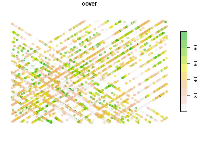
#> [1] 84.25 83.58 15.28 3.21 1.60 27.38Our data is now ready to go, so let’s display it on a map:
data_rs |>
  make_sf() |>
  dplyr::select(cover) |>
  plot(pal = function(...) terrain.colors(..., alpha = 0.5, rev=T),
       pch = 19)


