Note: This package is no longer being actively maintained! I will still try to answer questions, but as dependencies get updated some things might get buggy as time passes. I recommend looking into Amy Kuceyeski's NeMo tool instead (https://github.com/kjamison/nemo)
LQT is an R implementation of the lesion quantification toolkit, based
on the paper “Lesion Quantification Toolkit: A MATLAB software tool for
estimating grey matter damage and white matter disconnections in
patients with focal brain
lesions”
by Griffis et al. The LQT is “a publicly available software package for
quantifying the structural impacts of focal brain lesions. It uses
atlas-based approaches to estimate parcel-level grey matter lesion loads
and multiple measures of white matter disconnection severity that
include tract-level disconnection measures, voxel-wise disconnection
maps, and parcel-wise disconnection matrices. The toolkit also estimates
lesion-induced increases in the lengths of the shortest structural paths
between parcel pairs, which provide information about changes in
higher-order structural network topology.”
The R package creates data structures necessary for applying the methods directly to MNI-registered lesion maps from either a single patient or a full study. The package then allows the user to create figures for visualization and summary, and to compile analysis-ready datasets for research.
To get the latest development version from GitHub:
devtools::install_github('jdwor/LQT')Below is a description of the included functions and their usage, alongside examples of how an analysis would be run from beginning to end. The repository also contains two example files (“Example_Multi_Patient_Script.R” and “Example_Single_Patient_Script.R”) that can be downloaded, edited, and run locally.
This function creates a configuration (cfg) object that contains relevant information on file locations, parcellation choices, and parameter options for downstream analyses. At minimum, the user specifies either a single patient ID or a vector of patient IDs, as well as either a single lesion mask file path or a vector of lesion mask file paths corresponding to the patient ID(s) and in MNI space. The user also specifies an output path to which results and images will be saved.
Additional options include ‘parcel_path’, which allows a user to specify a path to a 1mm MNI parcellation image, ‘file_suffix’, which allows a user to specify naming conventions for the output files, ‘node_label’ and ‘node_group’, which allow users to provide additional parcellation information (though these are automatically loaded when using the built-in Schaefer-Yeo atlases), as well as additional visualization and specification options (see ?create_cfg_object for more information).
########### Set up config structure ###########
pat_ids = paste0("Subject", 1:45)
lesion_paths = list.files('/Users/JaneGoodall/Study/LesionMasks',
                          full.names = TRUE)
parcel_path = system.file("extdata","Schaefer_Yeo_Plus_Subcort",
                          "100Parcels7Networks.nii.gz",package="LQT")
out_path = '/Users/JaneGoodall/Study/Results'

cfg = create_cfg_object(pat_ids=pat_ids,
                        lesion_paths=lesion_paths,
                        parcel_path=parcel_path,
out_path=out_path)This function takes a pre-built cfg object and estimates the amount of damage sustained by each brain region. Regions are defined by the parcellation file path provided in ‘create_cfg_object’. The cfg object is the only input to this function, and the desired number of cores can be specified if the cfg object includes multiple subjects. The function saves three files to the output directory, 1) a nifti lesion mask, 2) a nifti damage map, giving the % of each parcel that overlapped lesion voxels, and 3) a csv with the percent damage to each parcel.
This function computes tract-based disconnection measures, with tracts defined by the HCP-842 tractography atlas as described in Yeh et al., (2018 - NeuroImage). The cfg object is the only input to this function, and the desired number of cores can be specified if the cfg object includes multiple subjects. The function saves one file to the output directory, a csv with the (probabilistic) % disconnection of each tract.
This is a wrapper that calls a series of functions to create various parcel disconnection measures. It wraps the ‘get_parcel_atlas’, ‘get_atlas_sspl’, ‘get_parcel_discon’, and ‘get_patient_sspl’ functions, checking whether atlas connectivity measures have been calculated and then running the study-specific disconnectivity assessments. This function creates four directories: “Atlas” - containing connectivity matrices and measures based on the given parcellation and the HCP 842 tracts; “Parcel_Disconnection” - containing patient-specific matrices and measures of probabilistic lesion-based disconnectivity between parcels; “Parcel_SSPL” - containing patient-specific matrices of increased structural shortest path length between parcels; and “Disconnection_Maps” - containing nifti images showing voxel-level and streamline-level disconnectivity.
########### Create Damage and Disconnection Measures ###########
# Get parcel damage for patients
get_parcel_damage(cfg, cores=2)
# Get tract SDC for patients
get_tract_discon(cfg, cores=2)
# Get parcel SDC and SSPL measures for patients
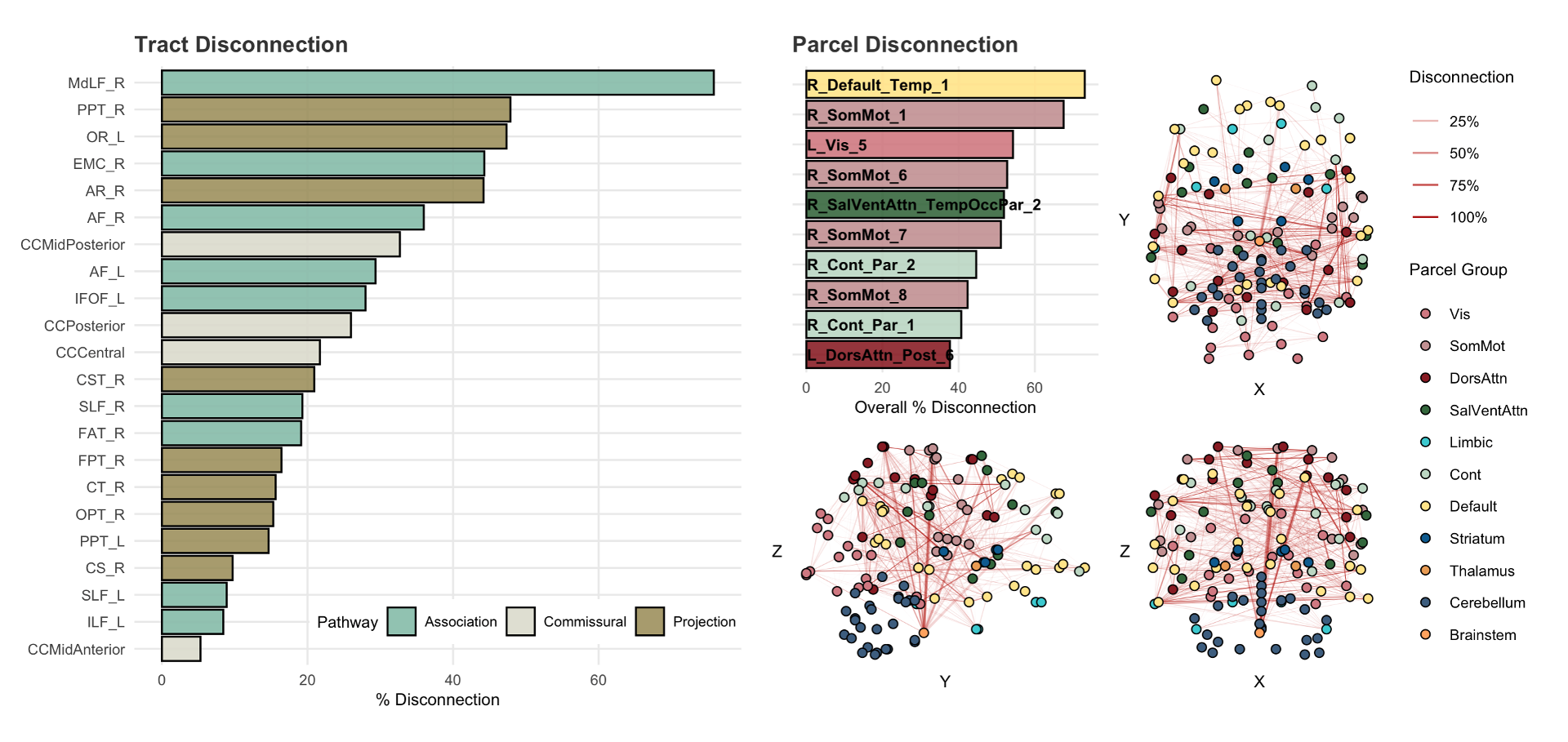
get_parcel_cons(cfg, cores=2)This function constructs subject-level visualizations of lesion-based damage and disconnection. For cfg objects with a single subject, the user only needs to specify the plot type. For cfg objects with multiple subjects, the user needs to specify the ID of the desired subject (or their numeric index) as well as the plot type. Plot type options are “parcel.damage”, which gives a barplot of percent parcel damage; “tract.discon”, which gives a barplot of percent tract-level disconnection; “parcel.discon”, which gives a barplot and brain network plots showing parcel-level disconnection; and “parcel.sspl”, which gives a barplot and brain network plots showing parcel-level structural shortest path length increases.
########### Build and View Summary Plots ###########
plot_lqt_subject(cfg, "Subject1", "parcel.damage")
plot_lqt_subject(cfg, "Subject1", "tract.discon")
plot_lqt_subject(cfg, "Subject1", "parcel.discon")
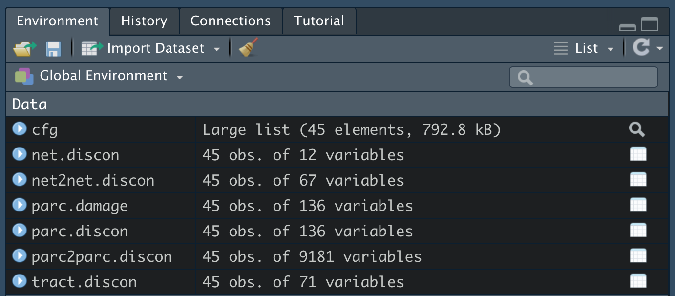
plot_lqt_subject(cfg, "Subject1", "parcel.sspl")This function reads in completed LQT results files and compiles analysis-ready datasets. The user provides the relevant config object (cfg), and can additionally specify the number of cores for the function to be run on. The function returns a list object containing several analysis-ready datasets, in which rows represent patients and columns represent lesion metrics: “parc.damage”, which gives percent regional parcel damage across subjects; “tract.discon”, which gives percent tract disconnection across subjects; “net.discon”, which gives the percent disconnection for each parcel group or network across its edges; “parc.discon”, which gives the percent disconnection for each individual parcel across its edges; “net2net.discon”, which gives the percent disconnection of each pairwise network-to-network edge; “parc2parc.discon”, which gives the percent disconnection of each pairwise parcel-to-parcel edge. These datasets each contain an ID column to facilitate merging with clinical data. Note that some of these datasets will have many columns, and some columns might have very little (or no) variance across subjects.
########### Compile Datasets for Analysis ###########
data = compile_data(cfg, cores = 2)
list2env(data, .GlobalEnv); rm(data)
There you have it! Good luck with your research, and don’t hesitate to email me at jordan.dworkin [at] nyspi [dot] columbia [dot] edu if you have any questions about the package.

