This package implements various tests, visualizations, and metrics for use with environmental niche models (ENMs) and species distribution models (SDMs).
At present, ENMTools is downloadable from https://github.com/danlwarren/ENMTools. There are multiple ways to download it. The easiest is to use devtools and install from GitHub.
Run the following code from your R console:
install.packages("devtools")
library(devtools)
install_github("danlwarren/ENMTools")
library(ENMTools)
A zipped version of the package is available at https://github.com/danlwarren/ENMTools/archive/master.zip. To install from the zip file, download a copy of it to your system. Once it's finished downloading, type the following (where PATH is the path to the zip file):
install.packages("devtools")
library(devtools)
install_local("PATH")
library(ENMTools)
First we're going to load in some environmental data.
env.files <- list.files(path = "test/testdata/", pattern = "pc", full.names = TRUE)
env <- stack(env.files)
names(env) <- c("pc1", "pc2", "pc3", "pc4")
env <- setMinMax(env)
ENMTools is primarily designed to examine patterns of similarity and difference between ENMs for different species. In order to simplify interactions with the functions in ENMTools, you need to put your data for each of your species into an enmtools.species object. You can create and view an empty enmtools.species object just by typing:
ahli <- enmtools.species()
ahli

##
##
## Range raster not defined.
##
## Presence points not defined.
##
## Background points not defined.
##
## Species name not defined.
You can add data to this object manually:
names(ahli)

## [1] "range"             "presence.points"   "background.points"
## [4] "models"            "species.name"

ahli$species.name <- "ahli"
ahli$presence.points <- read.csv("./test/testdata/ahli.csv")[,2:3]
ahli$range <- background.raster.buffer(ahli$presence.points, 50000, mask = env)
ahli$background.points <- background.points.buffer(points = ahli$presence.points,
                                                   radius = 20000, n = 1000, mask = env[[1]])

ahli

##
##
## Range raster:
## class       : RasterLayer
## dimensions  : 418, 1535, 641630  (nrow, ncol, ncell)
## resolution  : 0.008333333, 0.008333333  (x, y)
## extent      : -86.90809, -74.11642, 19.80837, 23.2917  (xmin, xmax, ymin, ymax)
## coord. ref. : NA
## data source : in memory
## names       : pc1
## values      : 1, 1  (min, max)
##
##
##
## Presence points (first ten only):
##
##  Longitude   Latitude
## ----------  ---------
##   -80.0106    21.8744
##   -79.9086    21.8095
##   -79.8065    21.7631
##   -79.8251    21.8095
##   -79.8807    21.8374
##   -79.9550    21.8374
##   -80.3446    22.0136
##   -80.2983    21.9951
##   -80.1776    21.9023
##   -80.1591    21.9673
##
##
## Background points (first ten only):
##
##  Longitude   Latitude
## ----------  ---------
##  -80.14559   22.16254
##  -80.35392   22.12087
##  -79.87059   22.00420
##  -80.05392   22.02087
##  -80.40392   22.17087
##  -79.97892   21.83754
##  -79.97059   22.08754
##  -80.08726   22.13754
##  -80.25392   22.01254
##  -80.31226   21.99587
##
##
## Species name:  ahli
Or you can add bits of it when the object is created:
allogus <- enmtools.species(species.name = "allogus",
                            presence.points = read.csv("./test/testdata/allogus.csv")[,3:4])

allogus$range <- background.raster.buffer(allogus$presence.points, 50000, mask = env)
allogus$background.points <- background.points.buffer(points = allogus$presence.points,
                                                      radius = 20000, n = 1000, mask = env[[1]])

allogus

##
##
## Range raster:
## class       : RasterLayer
## dimensions  : 418, 1535, 641630  (nrow, ncol, ncell)
## resolution  : 0.008333333, 0.008333333  (x, y)
## extent      : -86.90809, -74.11642, 19.80837, 23.2917  (xmin, xmax, ymin, ymax)
## coord. ref. : NA
## data source : in memory
## names       : pc1
## values      : 1, 1  (min, max)
##
##
##
## Presence points (first ten only):
##
##  Longitude   Latitude
## ----------  ---------
##   -79.2527    22.2109
##   -78.7774    22.2241
##   -78.6189    22.2373
##   -78.1039    21.1809
##   -78.0247    21.1809
##   -77.9983    20.9301
##   -77.9719    21.7091
##   -77.9719    21.5507
##   -77.9323    21.6167
##   -77.9323    20.7320
##
##
## Background points (first ten only):
##
##  Longitude   Latitude
## ----------  ---------
##  -76.07892   20.12087
##  -75.22892   20.49587
##  -77.93726   20.93754
##  -75.88726   20.23754
##  -77.86226   21.17920
##  -76.40392   20.37087
##  -78.05392   21.28754
##  -76.86226   20.72920
##  -77.85392   21.72087
##  -78.92059   22.25420
##
##
## Species name:  allogus
However, ENMTools also contains some sample data. It contains an enmtools.clade object called "iberolacerta.clade", which holds several enmtools.species objects. It also has some low-resolution Worldclim data that we can use to demonstrate functions. We'll pull two of those species out now.
data(iberolacerta.clade)
data(euro.worldclim)
monticola <- iberolacerta.clade$species$monticola
cyreni <- iberolacerta.clade$species$cyreni
env <- euro.worldclim
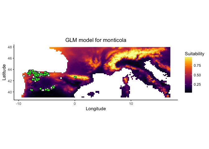
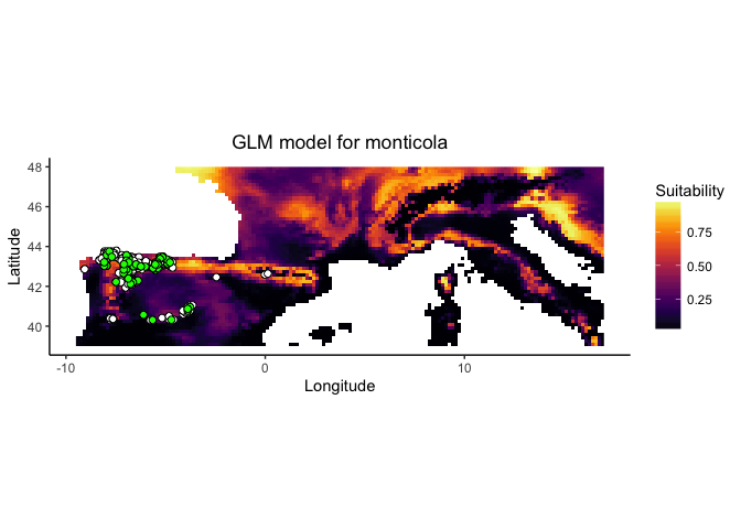
ENMTools contains functions to simplify the ENM construction process. Using enmtools.species objects and the correct modeling commands, we can build models very quickly. These commands are primarily wrappers to dismo model construction and projection functions, and at present are only available for GLM, Maxent, Domain, and Bioclim models. One of the nice bits about this setup is that it allows enmtools to automatically generate suitability maps, do model evaluation, and plot the marginal suitability of habitat for each variable separately.
Before we get started modeling, however, we might want to trim our predictor set so as to reduce collinearity. ENMTools contains a couple of handy functions for this.
raster.cor.matrix(env)

##              bio1         bio2        bio3        bio4       bio5
## bio1   1.00000000  0.208715969  0.36766171 -0.21357041  0.8853513
## bio2   0.20871597  1.000000000  0.58362743  0.30918934  0.5417192
## bio3   0.36766171  0.583627431  1.00000000 -0.56601419  0.3052211
## bio4  -0.21357041  0.309189341 -0.56601419  1.00000000  0.1754180
## bio5   0.88535133  0.541719174  0.30522110  0.17541802  1.0000000
## bio6   0.93295069 -0.017231880  0.42521254 -0.52131150  0.6875177
## bio7  -0.05329392  0.709020870 -0.14900115  0.87998888  0.4016817
## bio8   0.24945265  0.068562982 -0.16262988  0.30400935  0.2862188
## bio9   0.73849291  0.183148800  0.42195497 -0.37866158  0.6400464
## bio10  0.96045067  0.311324869  0.21975162  0.06247355  0.9606340
## bio11  0.95921479  0.101719882  0.48107648 -0.47305206  0.7533941
## bio12 -0.60846674 -0.482731496 -0.31488066 -0.07961919 -0.7137513
## bio13 -0.41433559 -0.510317568 -0.25626002 -0.19124801 -0.5722885
## bio14 -0.72871981 -0.338229901 -0.37618609  0.16712793 -0.7297745
## bio15  0.45421260 -0.007931916  0.11838593 -0.21759678  0.3821863
## bio16 -0.44597594 -0.506032477 -0.26995545 -0.16924912 -0.5920746
## bio17 -0.70338945 -0.343806007 -0.33935275  0.10832583 -0.7243068
## bio18 -0.81091065 -0.331213024 -0.47078459  0.28348226 -0.7776879
## bio19 -0.12414066 -0.396445432  0.07348362 -0.48121938 -0.3430162
##              bio6        bio7        bio8       bio9       bio10
## bio1   0.93295069 -0.05329392  0.24945265  0.7384929  0.96045067
## bio2  -0.01723188  0.70902087  0.06856298  0.1831488  0.31132487
## bio3   0.42521254 -0.14900115 -0.16262988  0.4219550  0.21975162
## bio4  -0.52131150  0.87998888  0.30400935 -0.3786616  0.06247355
## bio5   0.68751772  0.40168174  0.28621877  0.6400464  0.96063401
## bio6   1.00000000 -0.38884596  0.09285337  0.7734384  0.80726704
## bio7  -0.38884596  1.00000000  0.24603268 -0.1633540  0.20071994
## bio8   0.09285337  0.24603268  1.00000000 -0.2200483  0.33135353
## bio9   0.77343845 -0.16335400 -0.22004834  1.0000000  0.66175815
## bio10  0.80726704  0.20071994  0.33135353  0.6617581  1.00000000
## bio11  0.98896057 -0.29134540  0.12985480  0.7886188  0.84907884
## bio12 -0.48704454 -0.29133189 -0.30622476 -0.4629735 -0.65829840
## bio13 -0.28138429 -0.37121605 -0.19351156 -0.3074562 -0.48860809
## bio14 -0.67564389 -0.07381576 -0.25699492 -0.6265099 -0.71411350
## bio15  0.47445069 -0.11344874  0.17648853  0.3970693  0.41693023
## bio16 -0.31485467 -0.35410914 -0.21747973 -0.3274923 -0.51511693
## bio17 -0.63769389 -0.11473790 -0.30488093 -0.5552129 -0.70368996
## bio18 -0.80126262  0.02381502  0.03291308 -0.8163353 -0.76592247
## bio19  0.07715578 -0.53249335 -0.51356967  0.1072073 -0.26914814
##             bio11       bio12      bio13       bio14        bio15
## bio1   0.95921479 -0.60846674 -0.4143356 -0.72871981  0.454212596
## bio2   0.10171988 -0.48273150 -0.5103176 -0.33822990 -0.007931916
## bio3   0.48107648 -0.31488066 -0.2562600 -0.37618609  0.118385927
## bio4  -0.47305206 -0.07961919 -0.1912480  0.16712793 -0.217596785
## bio5   0.75339408 -0.71375135 -0.5722885 -0.72977455  0.382186338
## bio6   0.98896057 -0.48704454 -0.2813843 -0.67564389  0.474450688
## bio7  -0.29134540 -0.29133189 -0.3712161 -0.07381576 -0.113448735
## bio8   0.12985480 -0.30622476 -0.1935116 -0.25699492  0.176488534
## bio9   0.78861884 -0.46297347 -0.3074562 -0.62650986  0.397069264
## bio10  0.84907884 -0.65829840 -0.4886081 -0.71411350  0.416930231
## bio11  1.00000000 -0.54163405 -0.3297284 -0.72423144  0.492885864
## bio12 -0.54163405  1.00000000  0.9064818  0.77619752 -0.243139096
## bio13 -0.32972845  0.90648180  1.0000000  0.48404051  0.130409758
## bio14 -0.72423144  0.77619752  0.4840405  1.00000000 -0.743674332
## bio15  0.49288586 -0.24313910  0.1304098 -0.74367433  1.000000000
## bio16 -0.36513899  0.91789736  0.9902335  0.50120043  0.124449153
## bio17 -0.68356379  0.80791339  0.5245850  0.98592339 -0.729480228
## bio18 -0.82992875  0.76402046  0.5883523  0.84673991 -0.462267795
## bio19  0.01511498  0.74717071  0.7906993  0.31690226  0.128299899
##            bio16      bio17       bio18       bio19
## bio1  -0.4459759 -0.7033895 -0.81091065 -0.12414066
## bio2  -0.5060325 -0.3438060 -0.33121302 -0.39644543
## bio3  -0.2699555 -0.3393528 -0.47078459  0.07348362
## bio4  -0.1692491  0.1083258  0.28348226 -0.48121938
## bio5  -0.5920746 -0.7243068 -0.77768793 -0.34301616
## bio6  -0.3148547 -0.6376939 -0.80126262  0.07715578
## bio7  -0.3541091 -0.1147379  0.02381502 -0.53249335
## bio8  -0.2174797 -0.3048809  0.03291308 -0.51356967
## bio9  -0.3274923 -0.5552129 -0.81633533  0.10720732
## bio10 -0.5151169 -0.7036900 -0.76592247 -0.26914814
## bio11 -0.3651390 -0.6835638 -0.82992875  0.01511498
## bio12  0.9178974  0.8079134  0.76402046  0.74717071
## bio13  0.9902335  0.5245850  0.58835234  0.79069926
## bio14  0.5012004  0.9859234  0.84673991  0.31690226
## bio15  0.1244492 -0.7294802 -0.46226779  0.12829990
## bio16  1.0000000  0.5362200  0.61586400  0.79209065
## bio17  0.5362200  1.0000000  0.81764699  0.38396995
## bio18  0.6158640  0.8176470  1.00000000  0.17654879
## bio19  0.7920907  0.3839700  0.17654879  1.00000000
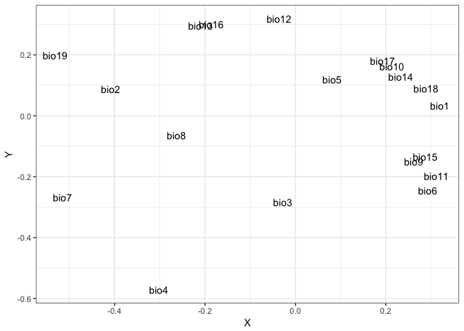
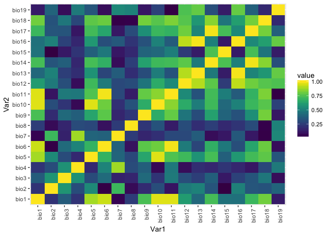
That's great, but it's a bit hard to pick variables this way. Let's try it visually instead.
raster.cor.plot(env)

## $cor.mds.plot
##
## $cor.heatmap
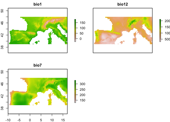
The raster.cor.plot function gives us two visualizations. One heatmap that colors pairs of predictors by their Pearson correlation coefficient, and one cluster plot that does mds scaling of the predictor variables and then plots them in a two dimensional space so that more correlated predictors are closer to each other. We're going to make an arbitrary decision to just use three predictors, and to keep those predictors relatively uncorrelated we'll select predictors that are far apart in this mds plot. Here we'll choose bio1, bio12, and bio7.
env <- env[[c("bio1", "bio12", "bio7")]]
plot(env)
raster.cor.matrix(env)

##              bio1      bio12        bio7
## bio1   1.00000000 -0.6084667 -0.05329392
## bio12 -0.60846674  1.0000000 -0.29133189
## bio7  -0.05329392 -0.2913319  1.00000000
GLMs usually require the user to supply a formula, an enmtools.species object, and some environmental data. If your formula is a strictly additive function of all of the environmental layers in env, though, enmtools.glm will build a formula automatically.
monticola.glm <- enmtools.glm(species = monticola, env = env, f = pres ~ bio1 + bio12 + bio7, test.prop = 0.2)

##
##
## No background points provided, drawing background from range raster.
##
## Adding environmental data to species monticola
##  Processing presence points...
##  Processing background points...

monticola.glm

##
##
## Formula:  presence ~ bio1 + bio12 + bio7
## <environment: 0x7fdc2203aa70>
##
##
## Data table (top ten lines):
##
##       Longitude   Latitude   bio1   bio12   bio7   presence
## ---  ----------  ---------  -----  ------  -----  ---------
## 1     -5.171215   43.06957     78     917    249          1
## 2     -6.036635   43.02531     76    1012    246          1
## 3     -7.679727   40.38852    137    1143    247          1
## 4     -7.790437   40.30959    129    1231    242          1
## 6     -6.575039   42.91070     84    1012    247          1
## 7     -5.132756   43.49572    133     822    190          1
## 8     -7.787378   40.39362    137    1143    247          1
## 9     -4.941888   43.35310    128     843    194          1
## 10    -7.621731   40.34170    101    1514    229          1
## 11    -7.645674   40.36543    101    1514    229          1
##
##
## Model:
## Call:
## glm(formula = f, family = "binomial", data = analysis.df[, -c(1,
##     2)], weights = weights)
##
## Deviance Residuals:
##     Min       1Q   Median       3Q      Max
## -1.6439  -0.7903  -0.4959   0.8448   2.2629
##
## Coefficients:
##               Estimate Std. Error z value Pr(>|z|)
## (Intercept)  8.3089037  2.1931131   3.789 0.000151 ***
## bio1        -0.0342866  0.0065015  -5.274 1.34e-07 ***
## bio12        0.0003411  0.0007222   0.472 0.636701
## bio7        -0.0205783  0.0049710  -4.140 3.48e-05 ***
## ---
## Signif. codes:  0 '***' 0.001 '**' 0.01 '*' 0.05 '.' 0.1 ' ' 1
##
## (Dispersion parameter for binomial family taken to be 1)
##
##     Null deviance: 576.70  on 719  degrees of freedom
## Residual deviance: 507.23  on 716  degrees of freedom
## AIC: 249.05
##
## Number of Fisher Scoring iterations: 4
##
##
##
## Model fit (training data):  class          : ModelEvaluation
## n presences    : 208
## n absences     : 512
## AUC            : 0.7393705
## cor            : 0.3210289
## max TPR+TNR at : -0.01700272
##
##
## Environment space model fit (training data):  class          : ModelEvaluation
## n presences    : 208
## n absences     : 10000
## AUC            : 0.4276125
## cor            : -0.01447189
## max TPR+TNR at : 0.4956744
##
##
## Proportion of data wittheld for model fitting:  0.2
##
## Model fit (test data):  class          : ModelEvaluation
## n presences    : 52
## n absences     : 512
## AUC            : 0.6924579
## cor            : 0.162511
## max TPR+TNR at : -0.00580997
##
##
## Environment space model fit (test data):  class          : ModelEvaluation
## n presences    : 52
## n absences     : 10000
## AUC            : 0.4033269
## cor            : -0.01488643
## max TPR+TNR at : 0.4984725
##
##
## Suitability:
## class       : RasterLayer
## dimensions  : 54, 162, 8748  (nrow, ncol, ncell)
## resolution  : 0.1666667, 0.1666667  (x, y)
## extent      : -10, 17, 39, 48  (xmin, xmax, ymin, ymax)
## coord. ref. : +proj=longlat +datum=WGS84 +ellps=WGS84 +towgs84=0,0,0
## data source : in memory
## names       : layer
## values      : 0.02397329, 0.9972282  (min, max)
##
##
##
## Notes:
Notice this produces the same formula as:
monticola.glm <- enmtools.glm(species = monticola, env = env, test.prop = 0.2)

##
##
## No background points provided, drawing background from range raster.
##
## Adding environmental data to species monticola
##  Processing presence points...
##  Processing background points...

monticola.glm

##
##
## Formula:  presence ~ bio1 + bio12 + bio7
## <environment: 0x7fdc379fe9c8>
##
##
## Data table (top ten lines):
##
##       Longitude   Latitude   bio1   bio12   bio7   presence
## ---  ----------  ---------  -----  ------  -----  ---------
## 1     -5.171215   43.06957     78     917    249          1
## 2     -6.036635   43.02531     76    1012    246          1
## 3     -7.679727   40.38852    137    1143    247          1
## 4     -7.790437   40.30959    129    1231    242          1
## 7     -5.132756   43.49572    133     822    190          1
## 8     -7.787378   40.39362    137    1143    247          1
## 9     -4.941888   43.35310    128     843    194          1
## 11    -7.645674   40.36543    101    1514    229          1
## 12    -7.642539   40.36317    101    1514    229          1
## 13    -6.990000   42.57000    107     893    253          1
##
##
## Model:
## Call:
## glm(formula = f, family = "binomial", data = analysis.df[, -c(1,
##     2)], weights = weights)
##
## Deviance Residuals:
##     Min       1Q   Median       3Q      Max
## -1.6668  -0.7985  -0.4761   0.8251   2.2069
##
## Coefficients:
##               Estimate Std. Error z value Pr(>|z|)
## (Intercept)  9.7242692  2.2707882   4.282 1.85e-05 ***
## bio1        -0.0371990  0.0066838  -5.566 2.61e-08 ***
## bio12       -0.0000931  0.0007383  -0.126      0.9
## bio7        -0.0235477  0.0051508  -4.572 4.84e-06 ***
## ---
## Signif. codes:  0 '***' 0.001 '**' 0.01 '*' 0.05 '.' 0.1 ' ' 1
##
## (Dispersion parameter for binomial family taken to be 1)
##
##     Null deviance: 576.70  on 719  degrees of freedom
## Residual deviance: 505.19  on 716  degrees of freedom
## AIC: 245.69
##
## Number of Fisher Scoring iterations: 4
##
##
##
## Model fit (training data):  class          : ModelEvaluation
## n presences    : 208
## n absences     : 512
## AUC            : 0.7367131
## cor            : 0.3226584
## max TPR+TNR at : 0.06883724
##
##
## Environment space model fit (training data):  class          : ModelEvaluation
## n presences    : 208
## n absences     : 10000
## AUC            : 0.4251981
## cor            : -0.01381147
## max TPR+TNR at : 0.3610308
##
##
## Proportion of data wittheld for model fitting:  0.2
##
## Model fit (test data):  class          : ModelEvaluation
## n presences    : 52
## n absences     : 512
## AUC            : 0.7000826
## cor            : 0.1634975
## max TPR+TNR at : 0.07265669
##
##
## Environment space model fit (test data):  class          : ModelEvaluation
## n presences    : 52
## n absences     : 10000
## AUC            : 0.4120712
## cor            : -0.01234761
## max TPR+TNR at : 0.4952489
##
##
## Suitability:
## class       : RasterLayer
## dimensions  : 54, 162, 8748  (nrow, ncol, ncell)
## resolution  : 0.1666667, 0.1666667  (x, y)
## extent      : -10, 17, 39, 48  (xmin, xmax, ymin, ymax)
## coord. ref. : +proj=longlat +datum=WGS84 +ellps=WGS84 +towgs84=0,0,0
## data source : in memory
## names       : layer
## values      : 0.01949305, 0.9973357  (min, max)
##
##
##
## Notes:
If you want a more complicated formula, though (e.g., with interactions or polynomial effects), you'll need to supply that manually.
monticola.glm <- enmtools.glm(species = monticola, env = env, f = pres ~ poly(bio1, 2) + poly(bio7, 2) * poly(bio12, 2), test.prop = 0.2)

##
##
## No background points provided, drawing background from range raster.
##
## Adding environmental data to species monticola
##  Processing presence points...
##  Processing background points...

monticola.glm

##
##
## Formula:  presence ~ poly(bio1, 2) + poly(bio7, 2) + poly(bio12, 2) + poly(bio7,
##     2):poly(bio12, 2)
## <environment: 0x7fdc20831e60>
##
##
## Data table (top ten lines):
##
##       Longitude   Latitude   bio1   bio12   bio7   presence
## ---  ----------  ---------  -----  ------  -----  ---------
## 1     -5.171215   43.06957     78     917    249          1
## 2     -6.036635   43.02531     76    1012    246          1
## 3     -7.679727   40.38852    137    1143    247          1
## 4     -7.790437   40.30959    129    1231    242          1
## 5     -7.473340   43.78935    140     931    179          1
## 6     -6.575039   42.91070     84    1012    247          1
## 7     -5.132756   43.49572    133     822    190          1
## 8     -7.787378   40.39362    137    1143    247          1
## 10    -7.621731   40.34170    101    1514    229          1
## 11    -7.645674   40.36543    101    1514    229          1
##
##
## Model:
## Call:
## glm(formula = f, family = "binomial", data = analysis.df[, -c(1,
##     2)], weights = weights)
##
## Deviance Residuals:
##     Min       1Q   Median       3Q      Max
## -1.3269  -0.7112  -0.3866   0.6404   2.6673
##
## Coefficients:
##                                 Estimate Std. Error z value Pr(>|z|)
## (Intercept)                      -0.9591     0.4109  -2.334  0.01958 *
## poly(bio1, 2)1                  -30.6734     5.7687  -5.317 1.05e-07 ***
## poly(bio1, 2)2                  -32.4723     6.4276  -5.052 4.37e-07 ***
## poly(bio7, 2)1                  -16.7741    12.8116  -1.309  0.19043
## poly(bio7, 2)2                    5.8198    10.6370   0.547  0.58429
## poly(bio12, 2)1                  34.5309    12.6304   2.734  0.00626 **
## poly(bio12, 2)2                  -9.2282     9.7090  -0.950  0.34187
## poly(bio7, 2)1:poly(bio12, 2)1 -238.9043   440.0210  -0.543  0.58717
## poly(bio7, 2)2:poly(bio12, 2)1  -76.0475   291.2958  -0.261  0.79404
## poly(bio7, 2)1:poly(bio12, 2)2  624.6585   287.3713   2.174  0.02973 *
## poly(bio7, 2)2:poly(bio12, 2)2   99.7371   177.5479   0.562  0.57429
## ---
## Signif. codes:  0 '***' 0.001 '**' 0.01 '*' 0.05 '.' 0.1 ' ' 1
##
## (Dispersion parameter for binomial family taken to be 1)
##
##     Null deviance: 576.70  on 719  degrees of freedom
## Residual deviance: 448.36  on 709  degrees of freedom
## AIC: 238.89
##
## Number of Fisher Scoring iterations: 5
##
##
##
## Model fit (training data):  class          : ModelEvaluation
## n presences    : 208
## n absences     : 512
## AUC            : 0.7964524
## cor            : 0.4205467
## max TPR+TNR at : 0.1333889
##
##
## Environment space model fit (training data):  class          : ModelEvaluation
## n presences    : 208
## n absences     : 10000
## AUC            : 0.7314553
## cor            : 0.1168428
## max TPR+TNR at : 0.3741629
##
##
## Proportion of data wittheld for model fitting:  0.2
##
## Model fit (test data):  class          : ModelEvaluation
## n presences    : 52
## n absences     : 512
## AUC            : 0.7557843
## cor            : 0.2330202
## max TPR+TNR at : -0.08155348
##
##
## Environment space model fit (test data):  class          : ModelEvaluation
## n presences    : 52
## n absences     : 10000
## AUC            : 0.7097
## cor            : 0.0509356
## max TPR+TNR at : 0.2494423
##
##
## Suitability:
## class       : RasterLayer
## dimensions  : 54, 162, 8748  (nrow, ncol, ncell)
## resolution  : 0.1666667, 0.1666667  (x, y)
## extent      : -10, 17, 39, 48  (xmin, xmax, ymin, ymax)
## coord. ref. : +proj=longlat +datum=WGS84 +ellps=WGS84 +towgs84=0,0,0
## data source : in memory
## names       : layer
## values      : 2.220446e-16, 0.992979  (min, max)
##
##
##
## Notes:
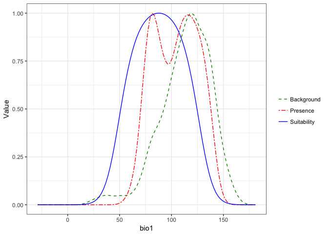
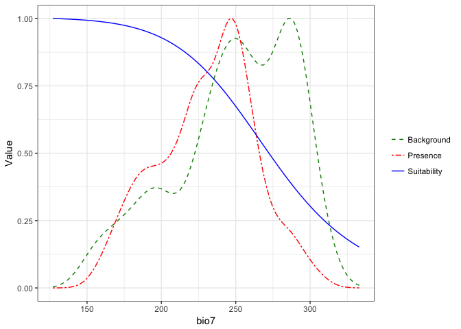
To check out the marginal response functions, you only need to type
monticola.glm$response.plots

## $bio1
##
## $bio7
##
## $bio12
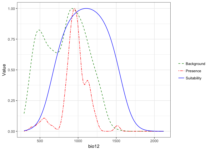
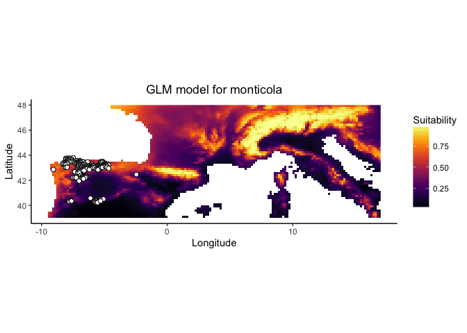
These plots present a smoothed estimate of the frequency of different levels of the environemntal variable in the presence data and the background points, along with the estimated relationship between that environmental predictor and the suitability of habitat from the model.
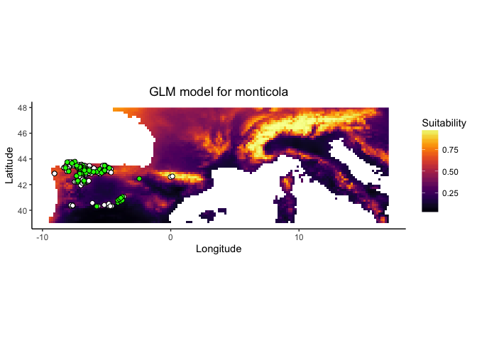
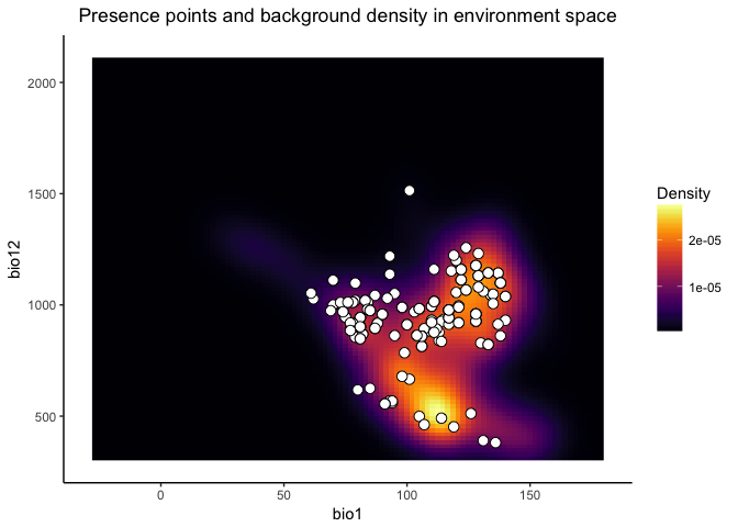
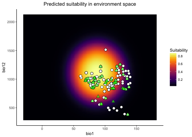
You can also visualize your models and data in a 2D environment space using any pair of layers from your environment stack. These plots hold all non-plotted variables (bio7 in this case) constant at their mean value across all presence points, then vary the plotted variables between the minimum and maximum values in env.
The suit.plot shows you suitability in environment space as a function of your two variables, with brighter colors representing variable combinations predicted to be more suitable. The points represent the occurrence points for your species in that environment space.
The colored raster of the background.plot shows you the density of background points in environment space, while the white points again represent your occurrence points in environment space.
visualize.enm(monticola.glm, env, layers = c("bio1", "bio12"), plot.test.data = TRUE)

## $background.plot
##
## $suit.plot
The procedure for building Bioclim, Domain, and Maxent models is similar to the procedure for GLMs, with the exception that you do not need to pass a formula to the model function for Maxent, Domain, and Bioclim models. Note that running Maxent models requires a bit of extra setup; see dismo documentation for details.
monticola.gam <- enmtools.gam(monticola, env, f = pres ~ poly(bio1, 2) + poly(bio7, 2) * poly(bio12, 2), test.prop = 0.2)
monticola.dm <- enmtools.dm(monticola, env, test.prop = 0.2)
monticola.bc <- enmtools.bc(monticola, env, test.prop = 0.2)
monticola.mx <- enmtools.maxent(monticola, env, test.prop = 0.2)
ENMTools provides a number of metrics for ENMs and for similarities between ENMs. These include measures of niche breadth, based on Levins(1968). An important caveat when interpreting these metrics is that they are driven to some (variable) extent by the availability of different combinations of environmental predictors. As such they are more accurately interpreted as a measurment of the smoothness of the geographic distribution of suitability scores than as an estimate of the breadth of the fundamental niche; an organism with narrow fundamental niche breadth that nonetheless encompasses a set of environmental conditions that is quite common will have a high breadth when measured using ENMs, while having a low breadth in environment space.
raster.breadth(monticola.glm)

## $B1
## [1] 0.9440004
##
## $B2
## [1] 0.5296247
ENMTools also provides metrics for measuring similarity between ENMs. These include Schoener's D (Schoener 1968), I (Warren et al. 2008), and the Spearman rank correlation coefficient between two rasters. While D and I are commonly used in the ENM literature, they may tend to overestimate similarity between ENMs when many grid cells are of similar values (e.g., when two species prefer different habitat but the region contains a great deal of habitat that is unsuitable for both).
monticola.glm <- enmtools.glm(species = monticola, env = env, f = pres ~ poly(bio1, 2) + poly(bio7, 2) + poly(bio12, 2), test.prop = 0.2)

##
##
## No background points provided, drawing background from range raster.
##
## Adding environmental data to species monticola
##  Processing presence points...
##  Processing background points...

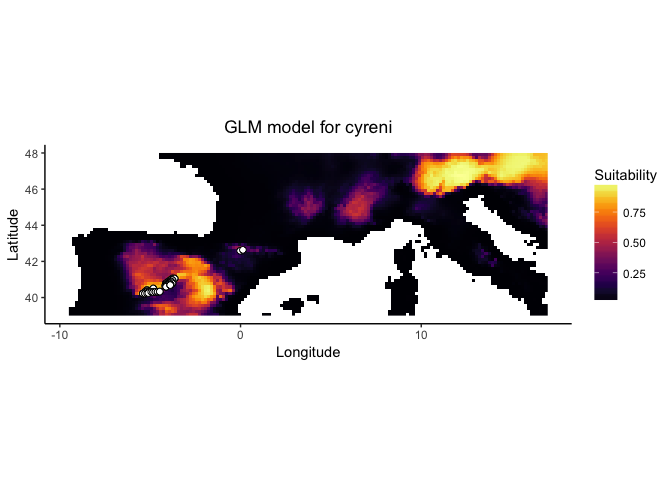
cyreni.glm <- enmtools.glm(species = cyreni, env = env, f = pres ~ poly(bio1, 2) + poly(bio7, 2) + poly(bio12, 2), test.prop = 0.2)

##
##
## No background points provided, drawing background from range raster.
##
## Adding environmental data to species cyreni
##  Processing presence points...
##  Processing background points...

raster.overlap(monticola.glm, cyreni.glm)

## $D
## [1] 0.6964057
##
## $I
## [1] 0.9026603
##
## $rank.cor
## [1] 0.3249225
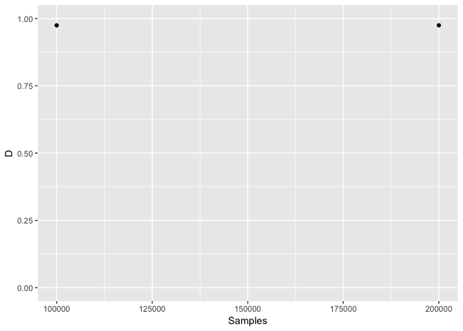
A new feature of the R version of ENMTools is that you can now use these same metrics in the n-dimensional space of all combinations of environmental variables, instead of restricting your measures of model similarity to those sets of conditions that appear in the training region. This is done by repeatedly drawing Latin hypercube samples from the space of all possible combinations of environmental variables given the min and max of each variable within the training region. ENMTools continues to draw samples until subsequent iterations differ by less than a specified tolerance value. Lower tolerance values result in more precise estimates of overlap, but can take much longer to calculate.
monticola.glm <- enmtools.glm(species = monticola, env = env, f = pres ~ poly(bio1, 2) + poly(bio7, 2) + poly(bio12, 2), test.prop = 0.2)

##
##
## No background points provided, drawing background from range raster.
##
## Adding environmental data to species monticola
##  Processing presence points...
##  Processing background points...

cyreni.glm <- enmtools.glm(species = monticola, env = env, f = pres ~ poly(bio1, 2) + poly(bio7, 2) + poly(bio12, 2), test.prop = 0.2)

##
##
## No background points provided, drawing background from range raster.
##
## Adding environmental data to species monticola
##  Processing presence points...
##  Processing background points...

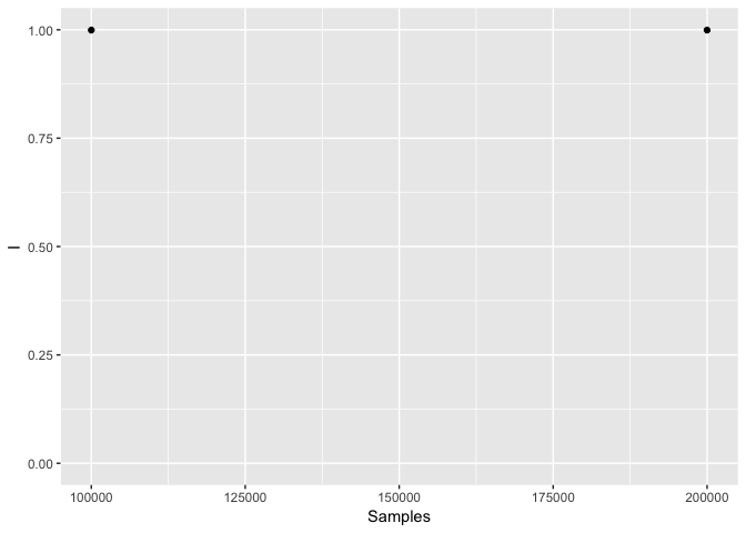
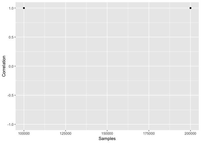
env.overlap(monticola.glm, cyreni.glm, env, tolerance = .001)

## [1] "Trying to find starting conditions, attempt 1"
## [1] "Building replicates..."

## $env.D
## [1] 0.9747509
##
## $env.I
## [1] 0.9992639
##
## $env.cor
## [1] 0.999296
##
## $env.D.plot
##
## $env.I.plot
##
## $env.cor.plot
The plots that come out of these environment space functions are used for diagnosing convergence of the overlap/breadth metric. Ideally what you want is a relationship between the metric and the number of samples that shows no clear directional trend.
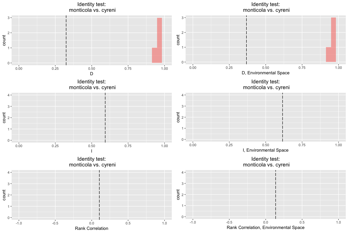
In this example, we will run a niche identity (also called equivalency) test, as in Warren et al. 2008. This test takes the presence points for a pair of species and randomly reassigns them to each species, then builds ENMs for these randomized occurrences. By doing this many times, we can estimate the probability distribution for ENM overlap between species under the null hypothesis that the two species' occurrences in the environment are effectively a random draw from the same underlying distribution. Note that niche evolution is only one of many reasons why two species' realized environmental distributions might cause departures from this null hypothesis. See Warren et al. 2014 for details.
To run an identity test, we need to decide what type of models we will build, how many replicates we will run, and (in the case of GLM and GAM) a model formula to use for empirical models and the Monte Carlo replicates. The resulting object contains the replicate models, p values, and plots of the results. Typically idenity tests are run with at least 99 replicates, but we are using a smaller number here for the sake of execution time.
NOTE: In order for models to be comparable, both empirical and pseudoreplicate models for the identity test are conducted with pseudoabsence points pooled for the two species being compared.
id.glm <- identity.test(species.1 = monticola, species.2 = cyreni, env = env, type = "glm", nreps = 4)

id.glm

##
##
##
##
## Identity test monticola vs. cyreni
##
## objectentity test p-values:
##        D        I rank.cor    env.D    env.I  env.cor
##      0.2      0.2      0.2      0.2      0.2      0.2
##
##
## Replicates:
##
##
##                      D           I    rank.cor       env.D       env.I     env.cor
## ----------  ----------  ----------  ----------  ----------  ----------  ----------
## empirical    0.3244487   0.5929443   0.1049357   0.3680675   0.6160525   0.1365335
## rep 1        0.9677634   0.9990155   0.9920496   0.9653146   0.9979226   0.9947297
## rep 2        0.9489356   0.9972812   0.9647560   0.9451813   0.9947636   0.9718006
## rep 3        0.9765731   0.9993665   0.9920094   0.9739029   0.9991720   0.9953646
## rep 4        0.9422789   0.9965344   0.9877409   0.9628450   0.9978574   0.9886635

## `stat_bin()` using `bins = 30`. Pick better value with `binwidth`.
## `stat_bin()` using `bins = 30`. Pick better value with `binwidth`.
## `stat_bin()` using `bins = 30`. Pick better value with `binwidth`.
## `stat_bin()` using `bins = 30`. Pick better value with `binwidth`.
## `stat_bin()` using `bins = 30`. Pick better value with `binwidth`.

## Warning: Removed 1 rows containing missing values (geom_bar).

## `stat_bin()` using `bins = 30`. Pick better value with `binwidth`.

## Warning: Removed 1 rows containing missing values (geom_bar).
The background or similarity test compares the overlap seen between two species' ENMs to the overlap expected by chance if one or both species was effectively choosing habitat at random from within their broad geographic range. The purpose of this test is to correct for the availability of habitat and ask whether the observed similarity between species or populations is significantly more (or less) than expected given the available set of environments in the regions in which they occur.
NOTE: In order for models to be comparable, both empirical and pseudoreplicate models for the background test are conducted with pseudoabsence points pooled for the two species being compared.
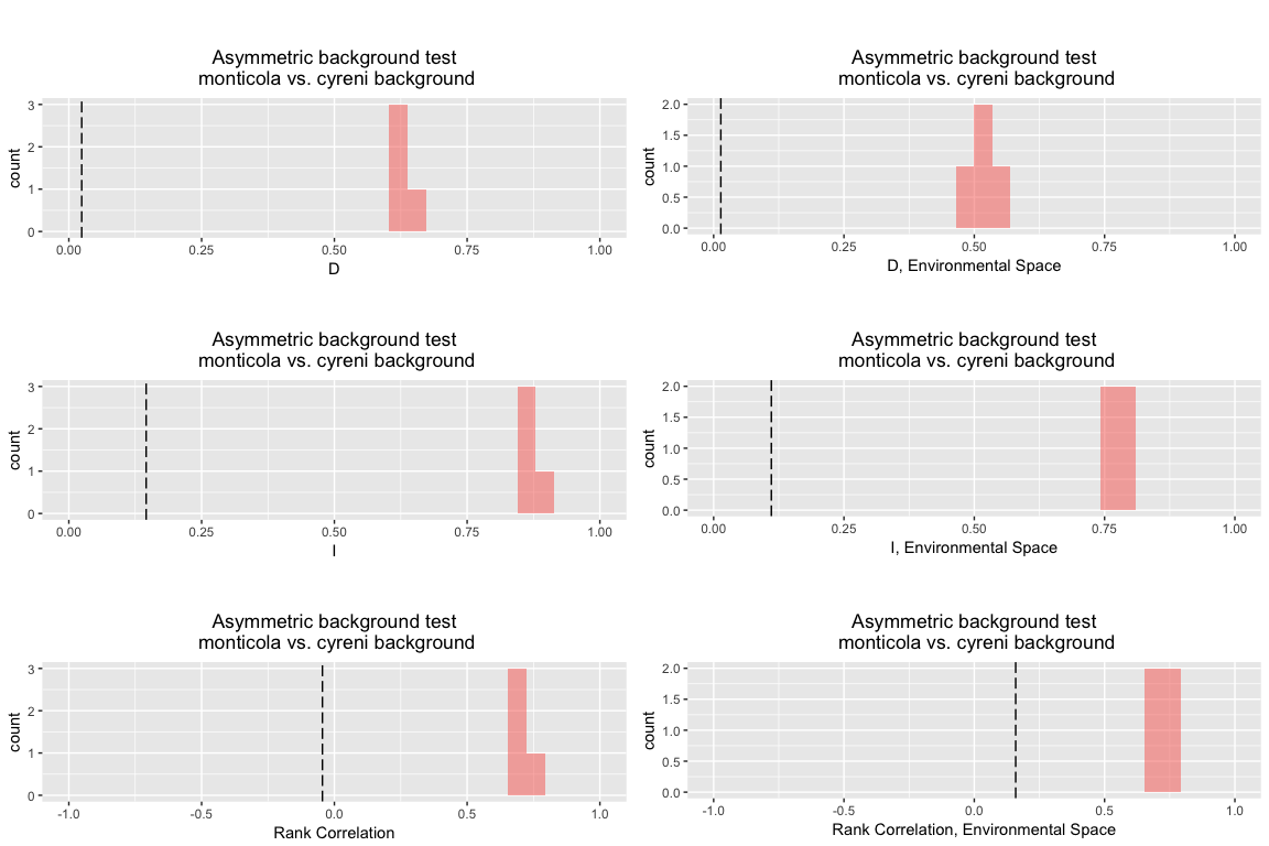
In Warren et al. 2008, we developed this test in the context of comparing one species' actual occurrence to the random background occurrences of the other species. This is what we call an "asymmetric" test, and in our case we did the test in both directions with the idea that we might compare the results of A vs. B background to the results of B vs. A background. This may be informative in some cases, but many people have also found this asymmetry confusing (and indeed it is often difficult to interpret). For that reason, the background test here can be conducted against a null hypothesis that is generated from "asymmetric" (species.1 vs species.2 background) or "symmetric" (species.1 background vs. species.2 background) comparisons.
Here, for instance, is a Bioclim background test using the classical asymmetric approach:
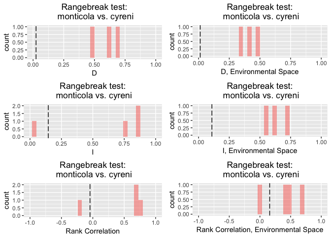
bg.bc.asym <- background.test(species.1 = monticola, species.2 = cyreni, env = env, type = "bc", nreps = 4, test.type = "asymmetric" )

bg.bc.asym

##
##
##
##
## Asymmetric background test
##  monticola vs. cyreni background
##
## background test p-values:
##        D        I rank.cor    env.D    env.I  env.cor
##      0.4      0.4      0.4      0.4      0.4      0.4
##
##
## Replicates:
##
##
##                      D           I     rank.cor       env.D       env.I     env.cor
## ----------  ----------  ----------  -----------  ----------  ----------  ----------
## empirical    0.0242365   0.1455829   -0.0450249   0.0138222   0.1107173   0.1589788
## rep 1        0.6214600   0.8700845    0.6715790   0.5110334   0.7742323   0.6747580
## rep 2        0.6140519   0.8692591    0.6881657   0.4890054   0.7671731   0.6784506
## rep 3        0.6477756   0.8921239    0.7362763   0.5359914   0.8078705   0.7271245
## rep 4        0.6349293   0.8741857    0.6796873   0.5338093   0.7872621   0.7335395

## `stat_bin()` using `bins = 30`. Pick better value with `binwidth`.
## `stat_bin()` using `bins = 30`. Pick better value with `binwidth`.
## `stat_bin()` using `bins = 30`. Pick better value with `binwidth`.
## `stat_bin()` using `bins = 30`. Pick better value with `binwidth`.
## `stat_bin()` using `bins = 30`. Pick better value with `binwidth`.

## Warning: Removed 1 rows containing missing values (geom_bar).

## `stat_bin()` using `bins = 30`. Pick better value with `binwidth`.

## Warning: Removed 1 rows containing missing values (geom_bar).
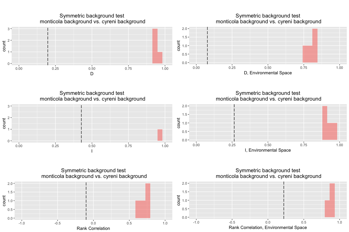
And here is a Domain background test using the symmetric approach:
bg.dm.sym <- background.test(species.1 = monticola, species.2 = cyreni, env = env, type = "dm", nreps = 4, test.type = "symmetric" )

bg.dm.sym

##
##
##
##
## Symmetric background test
##  monticola background vs. cyreni background
##
## background test p-values:
##        D        I rank.cor    env.D    env.I  env.cor
##      0.4      0.4      0.4      0.4      0.4      0.4
##
##
## Replicates:
##
##
##                      D           I     rank.cor       env.D       env.I     env.cor
## ----------  ----------  ----------  -----------  ----------  ----------  ----------
## empirical    0.1974048   0.4272913   -0.1020590   0.0775272   0.2648275   0.2207919
## rep 1        0.9462649   0.9964841    0.6346617   0.8440406   0.9521950   0.9254358
## rep 2        0.9546793   0.9976078    0.7412483   0.8426959   0.9476840   0.8970172
## rep 3        0.9213012   0.9824419    0.7453075   0.7434447   0.8853417   0.8458307
## rep 4        0.9407627   0.9926325    0.6575177   0.7768920   0.9123329   0.9387315

## `stat_bin()` using `bins = 30`. Pick better value with `binwidth`.
## `stat_bin()` using `bins = 30`. Pick better value with `binwidth`.
## `stat_bin()` using `bins = 30`. Pick better value with `binwidth`.
## `stat_bin()` using `bins = 30`. Pick better value with `binwidth`.
## `stat_bin()` using `bins = 30`. Pick better value with `binwidth`.

## Warning: Removed 1 rows containing missing values (geom_bar).

## `stat_bin()` using `bins = 30`. Pick better value with `binwidth`.

## Warning: Removed 1 rows containing missing values (geom_bar).
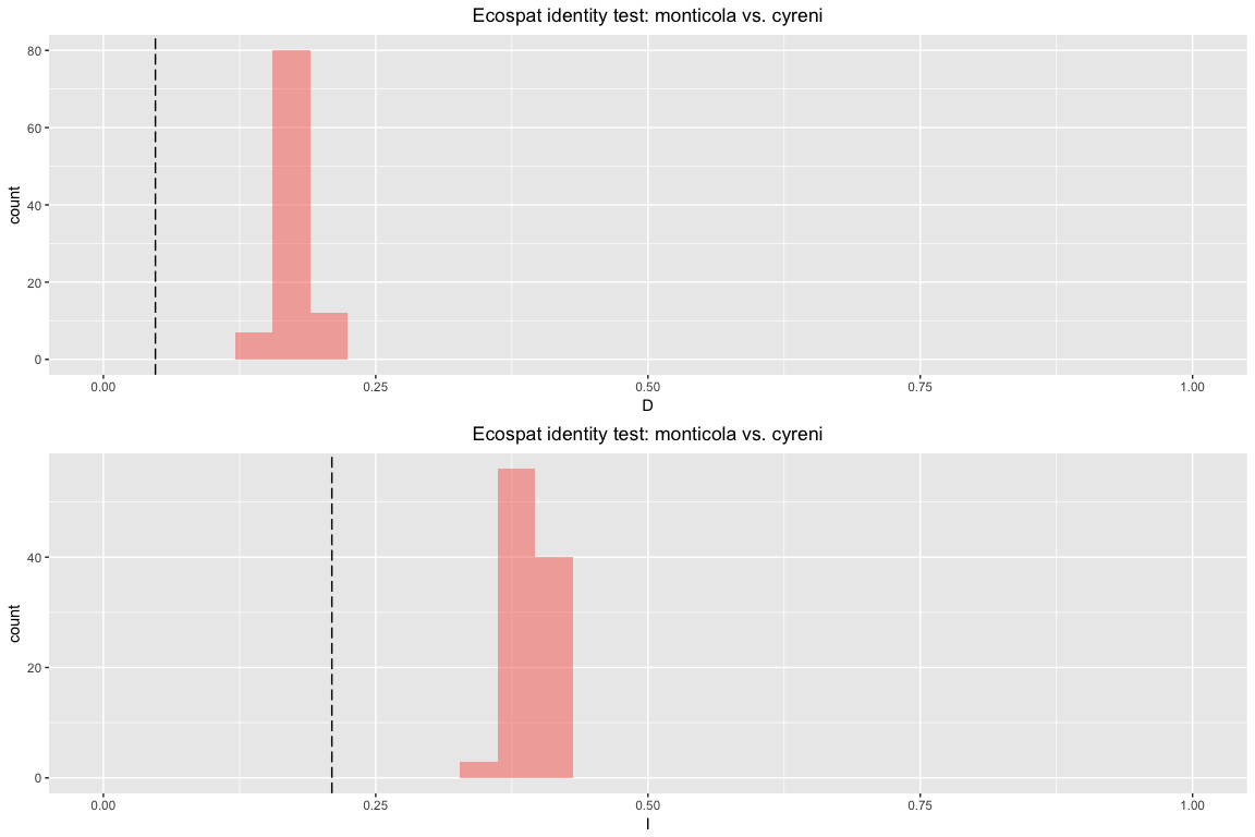
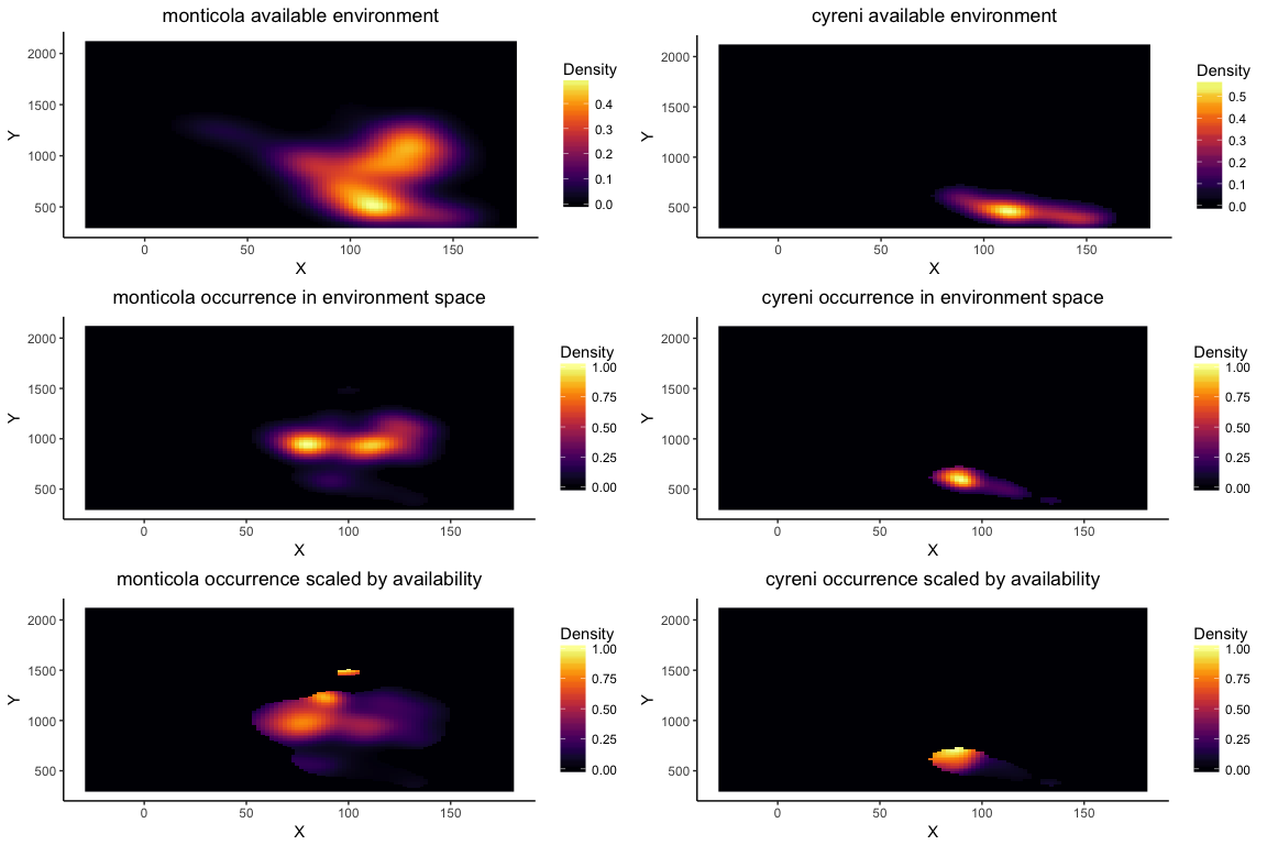
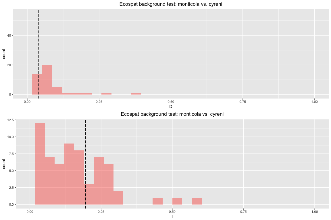
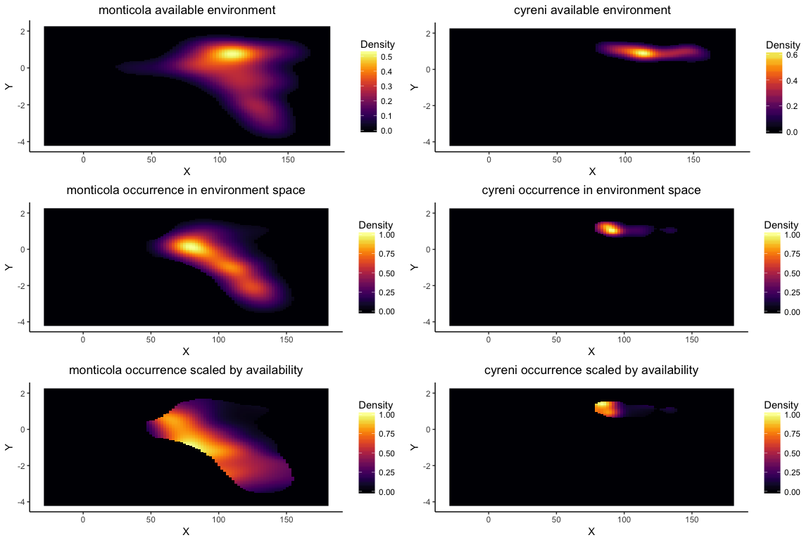
Using enmtools.species objects also provides a simplified interface to the niche equivalency and similarity tests (or identity and background tests, respectively) that were developed by Broennimann et al. (2012). These tests do not rely on ENMs, instead using kernel density smoothing to estimate density of the species in environment space. Ecospat also uses the density of the available environment to correct for availability when measuring overlaps, so that overlaps are not strictly driven by availability of combinations of environmental variables.
These tests only work with two environmental axes, so they are often done with the top two PC axes of a set of environments. In our case we'll just pick a couple of environmental layers, though (bio1 and bio2). Here's an equivalency/identity test:
esp.id <- enmtools.ecospat.id(monticola, cyreni, env[[c("bio1", "bio12")]])

##
##
## No background points provided, drawing background from range raster.
##
##
##
## No background points provided, drawing background from range raster.

esp.id

##
##
##
##
## Ecospat identity test monticola vs. cyreni
##
## ecospat.id test empirical overlaps:
## $D
## [1] 0.0477392
##
## $I
## [1] 0.2097866
##
##
##
## ecospat.id test p-values:
## D I
## 0 0

## `stat_bin()` using `bins = 30`. Pick better value with `binwidth`.
## `stat_bin()` using `bins = 30`. Pick better value with `binwidth`.
## NULL
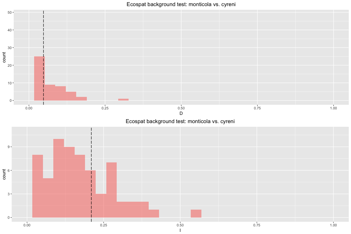
And here's a symmetric background test. The difference between symmetric and asymmetric for these tests is the same as for the background tests presented above.
esp.bg.sym <- enmtools.ecospat.bg(monticola, cyreni, env[[c("bio1", "bio12")]], test.type = "symmetric")

##
##
## No background points provided, drawing background from range raster.
##
##
##
## No background points provided, drawing background from range raster.

esp.bg.sym

##
##
##
##
## Ecospat background test symmetric monticola vs. cyreni
##
## ecospat.bg test empirical overlaps:
## $D
## [1] 0.0477392
##
## $I
## [1] 0.2097866
##
##
##
## ecospat.bg test p-values:
##    D    I
## 0.56 0.48

## `stat_bin()` using `bins = 30`. Pick better value with `binwidth`.
## `stat_bin()` using `bins = 30`. Pick better value with `binwidth`.

## Warning: Removed 24 rows containing non-finite values (stat_bin).
## NULL
Note that if you provide more than two layers to the enmtools.ecospat function, it will performa a PCA analysis on the provided layers and measure overlaps on the first two axes of that PCA space.
esp.bg.sym <- enmtools.ecospat.bg(monticola, cyreni, env, test.type = "symmetric")

##
##
## No background points provided, drawing background from range raster.
##
##
##
## No background points provided, drawing background from range raster.
##
## [1] "More than two layers in environment stack and no layers argument passed, performing PCA..."

esp.bg.sym

##
##
##
##
## Ecospat background test symmetric monticola vs. cyreni
##
## ecospat.bg test empirical overlaps:
## $D
## [1] 0.039695
##
## $I
## [1] 0.195018
##
##
##
## ecospat.bg test p-values:
##    D    I
## 0.64 0.44

## `stat_bin()` using `bins = 30`. Pick better value with `binwidth`.
## `stat_bin()` using `bins = 30`. Pick better value with `binwidth`.

## Warning: Removed 32 rows containing non-finite values (stat_bin).
## NULL
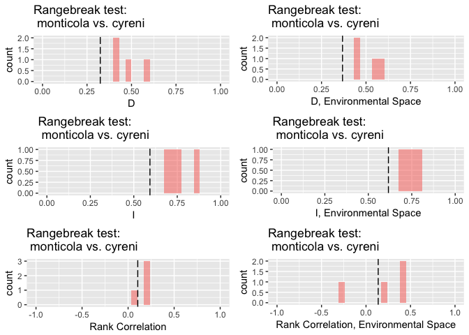
ENMTools also allows you to perform linear, blob, and ribbon rangebreak tests as developed in Glor and Warren 2011. The linear and blob tests are two versions of a test that permit one to ask whether the geographic regions occupied by two species are more environmentally different than expected by chance. The ribbon test, meanwhile, is designed to test whether the ranges of two species are divided by a region that is relatively unsuitable to one or both forms.
For the linear and blob tests, you call them very much like you would the identity and background tests. Here's a linear one using GLM models:
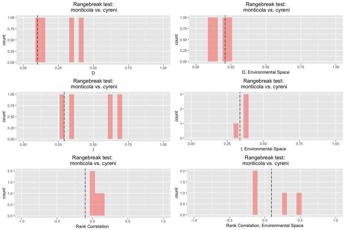
rbl.glm <- rangebreak.linear(monticola, cyreni, env, type = "glm", nreps = 4)

##
##
## No background points provided, drawing background from range raster.
##
##
##
## No background points provided, drawing background from range raster.
##
##
## Building empirical models...
## Adding environmental data to species monticola
##  Processing presence points...
##  Processing background points...
## Adding environmental data to species cyreni
##  Processing presence points...
##  Processing background points...
## [1] "Trying to find starting conditions, attempt 1"
## [1] "Building replicates..."
##
## Building replicate models...
##
## Replicate 1 ...
## Adding environmental data to species monticola
##  Processing presence points...
##  Processing background points...
## Adding environmental data to species cyreni
##  Processing presence points...
##  Processing background points...
## [1] "Trying to find starting conditions, attempt 1"
## [1] "Building replicates..."
##
## Replicate 2 ...
## Adding environmental data to species monticola
##  Processing presence points...
##  Processing background points...
## Adding environmental data to species cyreni
##  Processing presence points...
##  Processing background points...
## [1] "Trying to find starting conditions, attempt 1"
## [1] "Building replicates..."
##
## Replicate 3 ...
## Adding environmental data to species monticola
##  Processing presence points...
##  Processing background points...
## Adding environmental data to species cyreni
##  Processing presence points...
##  Processing background points...
## [1] "Trying to find starting conditions, attempt 1"
## [1] "Building replicates..."
##
## Replicate 4 ...
## Adding environmental data to species monticola
##  Processing presence points...
##  Processing background points...
## Adding environmental data to species cyreni
##  Processing presence points...
##  Processing background points...
## [1] "Trying to find starting conditions, attempt 1"
## [1] "Building replicates..."

rbl.glm

##
##
##
##
## Linear rangebreak test monticola vs. cyreni
##
## rangebreak test p-values:
##        D        I rank.cor    env.D    env.I  env.cor
##      0.2      0.2      0.4      0.2      0.2      0.4
##
##
## Replicates:
##
##
##                      D           I    rank.cor       env.D       env.I      env.cor
## ----------  ----------  ----------  ----------  ----------  ----------  -----------
## empirical    0.3244487   0.5929443   0.1049357   0.3682391   0.6158986    0.1370378
## rep 1        0.4164302   0.6969905   0.2230349   0.4452615   0.6985640    0.3871524
## rep 2        0.4221705   0.7136580   0.2200321   0.4554071   0.7113299    0.4364791
## rep 3        0.4723282   0.7568531   0.0458225   0.5744372   0.7832484    0.2085522
## rep 4        0.5971889   0.8541483   0.1981989   0.5651623   0.7668461   -0.2813777
## `stat_bin()` using `bins = 30`. Pick better value with `binwidth`.
## `stat_bin()` using `bins = 30`. Pick better value with `binwidth`.
## `stat_bin()` using `bins = 30`. Pick better value with `binwidth`.
## `stat_bin()` using `bins = 30`. Pick better value with `binwidth`.
## `stat_bin()` using `bins = 30`. Pick better value with `binwidth`.

## Warning: Removed 1 rows containing missing values (geom_bar).

## `stat_bin()` using `bins = 30`. Pick better value with `binwidth`.

## Warning: Removed 1 rows containing missing values (geom_bar).
And here's a blob test using Bioclim:
rbb.bc <- rangebreak.blob(monticola, cyreni, env, type = "bc", nreps = 4)

##
##
## No background points provided, drawing background from range raster.
##
##
##
## No background points provided, drawing background from range raster.
##
##
## Building empirical models...
## [1] "Trying to find starting conditions, attempt 1"
## [1] "Building replicates..."
##
## Building replicate models...
##
## Replicate 1 ...
## [1] "Trying to find starting conditions, attempt 1"
## [1] "Building replicates..."
##
## Replicate 2 ...
## [1] "Trying to find starting conditions, attempt 1"
## [1] "Building replicates..."
##
## Replicate 3 ...
## [1] "Trying to find starting conditions, attempt 1"
## [1] "Building replicates..."
##
## Replicate 4 ...
## [1] "Trying to find starting conditions, attempt 1"
## [1] "Building replicates..."

rbb.bc

##
##
##
##
## blob rangebreak test monticola vs. cyreni
##
## rangebreak test p-values:
##        D        I rank.cor    env.D    env.I  env.cor
##      0.4      0.4      0.4      0.4      0.4      0.4
##
##
## Replicates:
##
##
##                      D           I     rank.cor       env.D       env.I     env.cor
## ----------  ----------  ----------  -----------  ----------  ----------  ----------
## empirical    0.0242365   0.1455829   -0.0450249   0.0133100   0.1086260   0.1592556
## rep 1        0.6896760   0.8578952    0.7220233   0.4986668   0.7336902   0.7237154
## rep 2        0.0046566   0.0245867   -0.2164500   0.0019719   0.0132680   0.0017443
## rep 3        0.4882798   0.7556071    0.7118018   0.3291984   0.5505698   0.4024447
## rep 4        0.6220568   0.8484927    0.7545716   0.4055820   0.6054990   0.4720669

## `stat_bin()` using `bins = 30`. Pick better value with `binwidth`.
## `stat_bin()` using `bins = 30`. Pick better value with `binwidth`.
## `stat_bin()` using `bins = 30`. Pick better value with `binwidth`.
## `stat_bin()` using `bins = 30`. Pick better value with `binwidth`.
## `stat_bin()` using `bins = 30`. Pick better value with `binwidth`.

## Warning: Removed 1 rows containing missing values (geom_bar).

## `stat_bin()` using `bins = 30`. Pick better value with `binwidth`.

## Warning: Removed 1 rows containing missing values (geom_bar).
If you want to access the individual replicates (for instance to see how your ranges are being split up), you can find them in the list named "replicate.models" inside your rangebreak test object.
rbl.glm$replicate.models$monticola.rep.1

##
##
## Formula:  presence ~ bio1 + bio12 + bio7
## <environment: 0x7fdc11984fb8>
##
##
## Data table (top ten lines):
##
##  Longitude   Latitude   bio1   bio12   bio7   presence
## ----------  ---------  -----  ------  -----  ---------
##      -8.07      43.75    134    1045    166          1
##      -7.94      43.75    131    1061    171          1
##      -8.07      43.66    135    1048    168          1
##      -7.82      43.75    135    1006    174          1
##      -7.95      43.66    129    1080    176          1
##      -7.70      43.75    135    1006    174          1
##      -7.82      43.66    122    1113    184          1
##      -7.95      43.57    129    1080    176          1
##      -8.07      43.48    129    1131    178          1
##      -8.20      43.40    140    1038    164          1
##
##
## Model:
## Call:
## glm(formula = f, family = "binomial", data = analysis.df[, -c(1,
##     2)], weights = weights)
##
## Deviance Residuals:
##     Min       1Q   Median       3Q      Max
## -1.8790  -0.7547  -0.3902   0.7147   1.8858
##
## Coefficients:
##               Estimate Std. Error z value Pr(>|z|)
## (Intercept)  8.7745104  2.1895024   4.008 6.14e-05 ***
## bio1        -0.0409593  0.0065667  -6.237 4.45e-10 ***
## bio12        0.0011127  0.0007125   1.562    0.118
## bio7        -0.0217979  0.0048563  -4.489 7.17e-06 ***
## ---
## Signif. codes:  0 '***' 0.001 '**' 0.01 '*' 0.05 '.' 0.1 ' ' 1
##
## (Dispersion parameter for binomial family taken to be 1)
##
##     Null deviance: 720.87  on 901  degrees of freedom
## Residual deviance: 584.14  on 898  degrees of freedom
## AIC: 273.49
##
## Number of Fisher Scoring iterations: 5
##
##
##
## Model fit (training data):  class          : ModelEvaluation
## n presences    : 260
## n absences     : 642
## AUC            : 0.7830068
## cor            : 0.3935289
## max TPR+TNR at : -0.4716333
##
##
## Environment space model fit (training data):  class          : ModelEvaluation
## n presences    : 260
## n absences     : 10000
## AUC            : 0.4248523
## cor            : -0.008857617
## max TPR+TNR at : 0.3841534
##
##
## Proportion of data wittheld for model fitting:  0
##
## Model fit (test data):  [1] NA
##
##
## Environment space model fit (test data):  [1] NA
##
##
## Suitability:
## class       : RasterLayer
## dimensions  : 54, 162, 8748  (nrow, ncol, ncell)
## resolution  : 0.1666667, 0.1666667  (x, y)
## extent      : -10, 17, 39, 48  (xmin, xmax, ymin, ymax)
## coord. ref. : +proj=longlat +datum=WGS84 +ellps=WGS84 +towgs84=0,0,0
## data source : in memory
## names       : layer
## values      : 0.01243438, 0.9996217  (min, max)
##
##
##
## Notes:
rbl.glm$replicate.models$cyreni.rep.1

##
##
## Formula:  presence ~ bio1 + bio12 + bio7
## <environment: 0x7fdc3c89aee0>
##
##
## Data table (top ten lines):
##
##  Longitude   Latitude   bio1   bio12   bio7   presence
## ----------  ---------  -----  ------  -----  ---------
##      -5.18      40.41     85     625    294          1
##      -5.18      40.41     85     625    294          1
##      -5.29      40.31     89     646    296          1
##      -5.29      40.31     89     646    296          1
##      -5.17      40.36     85     625    294          1
##      -5.41      40.22     93     645    295          1
##      -5.41      40.22     93     645    295          1
##      -5.18      40.32     89     646    296          1
##      -4.83      40.50    107     462    298          1
##      -4.83      40.50    107     462    298          1
##
##
## Model:
## Call:
## glm(formula = f, family = "binomial", data = analysis.df[, -c(1,
##     2)], weights = weights)
##
## Deviance Residuals:
##     Min       1Q   Median       3Q      Max
## -0.7418  -0.3423  -0.1757  -0.0051   1.9055
##
## Coefficients:
##              Estimate Std. Error z value Pr(>|z|)
## (Intercept) -5.386065  10.904553  -0.494   0.6214
## bio1        -0.105238   0.019167  -5.491    4e-08 ***
## bio12       -0.006370   0.003437  -1.854   0.0638 .
## bio7         0.070905   0.033311   2.129   0.0333 *
## ---
## Signif. codes:  0 '***' 0.001 '**' 0.01 '*' 0.05 '.' 0.1 ' ' 1
##
## (Dispersion parameter for binomial family taken to be 1)
##
##     Null deviance: 210.72  on 847  degrees of freedom
## Residual deviance: 129.35  on 844  degrees of freedom
## AIC: 65.765
##
## Number of Fisher Scoring iterations: 7
##
##
##
## Model fit (training data):  class          : ModelEvaluation
## n presences    : 76
## n absences     : 772
## AUC            : 0.8721366
## cor            : 0.2682345
## max TPR+TNR at : -0.1611919
##
##
## Environment space model fit (training data):  class          : ModelEvaluation
## n presences    : 76
## n absences     : 10000
## AUC            : 0.8260658
## cor            : 0.1177308
## max TPR+TNR at : 0.31541
##
##
## Proportion of data wittheld for model fitting:  0
##
## Model fit (test data):  [1] NA
##
##
## Environment space model fit (test data):  [1] NA
##
##
## Suitability:
## class       : RasterLayer
## dimensions  : 54, 162, 8748  (nrow, ncol, ncell)
## resolution  : 0.1666667, 0.1666667  (x, y)
## extent      : -10, 17, 39, 48  (xmin, xmax, ymin, ymax)
## coord. ref. : +proj=longlat +datum=WGS84 +ellps=WGS84 +towgs84=0,0,0
## data source : in memory
## names       : layer
## values      : 1.15296e-08, 0.9931977  (min, max)
##
##
##
## Notes:
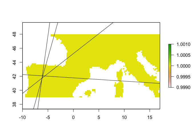
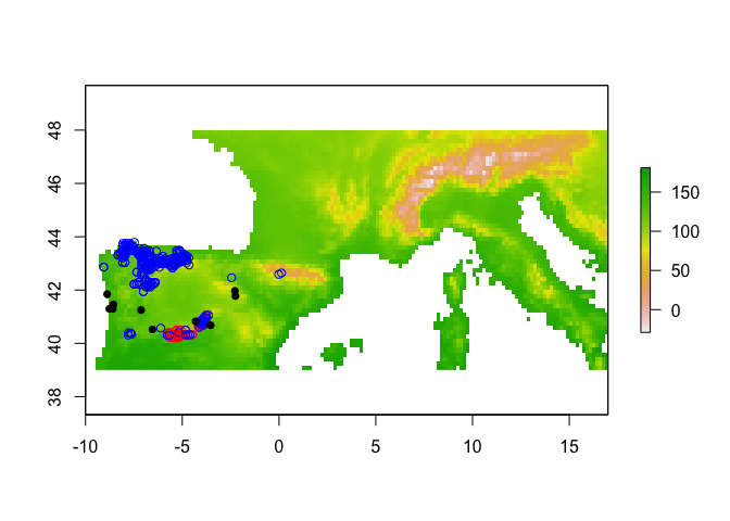
For the ribbon rangebreak test, you will need one extra thing; a third enmtools.species object representing the occurrence points (for one or both species) that fall within the ribbon of putatively unsuitable habitat. In the case of these two lizards we don't have such a ribbon, so we'll just simulate one based on some random points.
plot(env[[1]])
points(cyreni$presence.points, col = "red")
points(monticola$presence.points, col = "blue")

ribbon <- enmtools.species(species.name = "ribbon")
ribbon$presence.points <- data.frame(Longitude = runif(n = 10, min = -9, max = 0),
                                      Latitude = runif(n = 10, min = 40.5, max = 42))
points(ribbon$presence.points, pch = 16)
ribbon$range <- background.raster.buffer(ribbon$presence.points, 20000, mask = env)
ribbon

##
##
## Range raster:
## class       : RasterLayer
## dimensions  : 54, 162, 8748  (nrow, ncol, ncell)
## resolution  : 0.1666667, 0.1666667  (x, y)
## extent      : -10, 17, 39, 48  (xmin, xmax, ymin, ymax)
## coord. ref. : +proj=longlat +datum=WGS84 +ellps=WGS84 +towgs84=0,0,0
## data source : in memory
## names       : bio1
## values      : 1, 1  (min, max)
##
##
##
## Presence points (first ten only):
##
##  Longitude   Latitude
## ----------  ---------
##  -8.767481   41.29724
##  -7.129208   41.25078
##  -8.560360   41.45911
##  -2.252357   41.77763
##  -8.881490   41.84858
##  -6.539390   40.52293
##  -8.585099   41.29406
##  -4.308883   40.82632
##  -3.536658   40.67851
##  -2.280341   41.96987
##
##
## Background points not defined.
##
## Species name:  ribbon
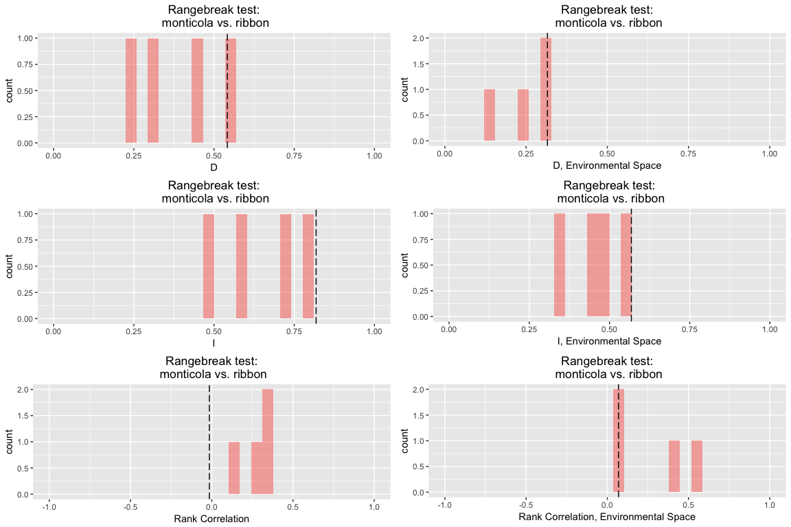
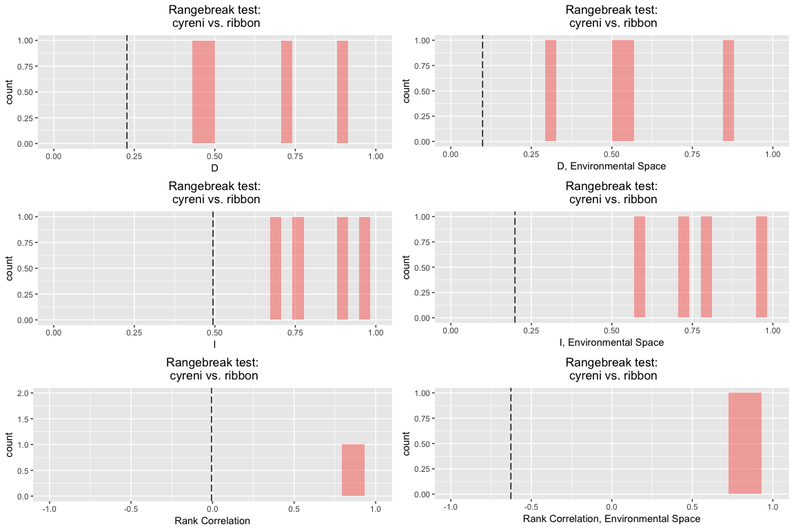
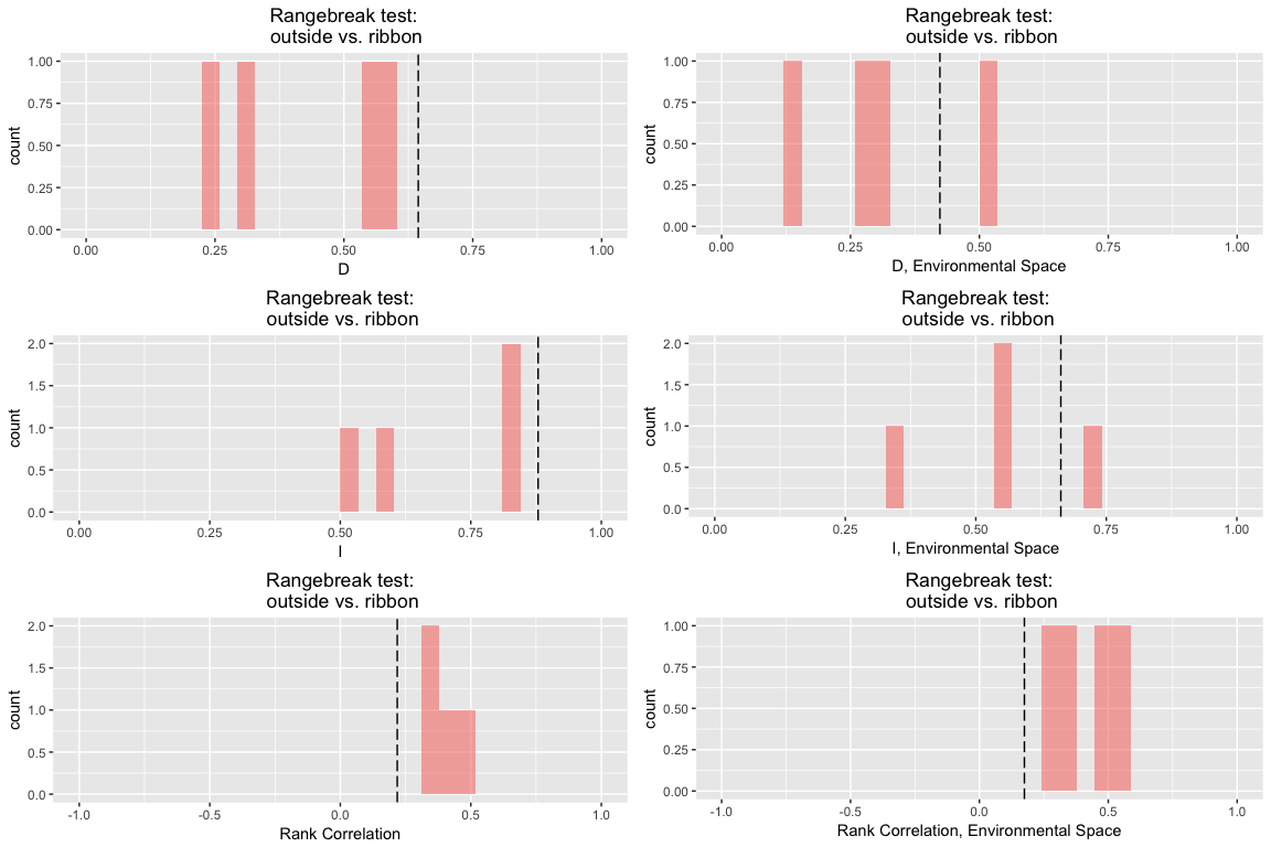
Now we'll run a ribbon rangebreak test using GLM models with quadratic effects. We also need to tell it the width of the ribbons to generate for the replicates. The units for the width argument are the same units that the presence points are in; e.g., if the points are in decimal degrees you should supply the width of the barrier in decimal degrees.
rbr.glm <- rangebreak.ribbon(monticola, cyreni, ribbon, env, type = "glm", f = pres ~ poly(bio1, 2) + poly(bio12, 2) + poly(bio7, 2), width = 0.5, nreps = 4)

##
##
## No background points provided, drawing background from range raster.
##
##
##
## No background points provided, drawing background from range raster.
##
##
##
## No background points provided, drawing background from range raster.
##
##
## Building empirical models...
## Adding environmental data to species monticola
##  Processing presence points...
##  Processing background points...
## Adding environmental data to species cyreni
##  Processing presence points...
##  Processing background points...

## Warning: glm.fit: fitted probabilities numerically 0 or 1 occurred

## Adding environmental data to species ribbon
##  Processing presence points...
##  Processing background points...
## Adding environmental data to species outside
##  Processing presence points...
##  Processing background points...
## [1] "Trying to find starting conditions, attempt 1"
## [1] "Building replicates..."
## [1] "Trying to find starting conditions, attempt 1"
## [1] "Building replicates..."
## [1] "Trying to find starting conditions, attempt 1"
## [1] "Building replicates..."
## [1] "Trying to find starting conditions, attempt 1"
## [1] "Building replicates..."
##
## Building replicate models...
##
## Replicate 1 ...
## Adding environmental data to species monticola
##  Processing presence points...
##  Processing background points...
## Adding environmental data to species cyreni
##  Processing presence points...
##  Processing background points...
## Adding environmental data to species ribbon
##  Processing presence points...
##  Processing background points...
## Adding environmental data to species outside
##  Processing presence points...
##  Processing background points...
## [1] "Trying to find starting conditions, attempt 1"
## [1] "Building replicates..."
## [1] "Trying to find starting conditions, attempt 1"
## [1] "Building replicates..."
## [1] "Trying to find starting conditions, attempt 1"
## [1] "Building replicates..."
## [1] "Trying to find starting conditions, attempt 1"
## [1] "Building replicates..."
##
## Replicate 2 ...
## Adding environmental data to species monticola
##  Processing presence points...
##  Processing background points...
## Adding environmental data to species cyreni
##  Processing presence points...
##  Processing background points...
## Adding environmental data to species ribbon
##  Processing presence points...
##  Processing background points...
## Adding environmental data to species outside
##  Processing presence points...
##  Processing background points...
## [1] "Trying to find starting conditions, attempt 1"
## [1] "Building replicates..."
## [1] "Trying to find starting conditions, attempt 1"
## [1] "Building replicates..."
## [1] "Trying to find starting conditions, attempt 1"
## [1] "Building replicates..."
## [1] "Trying to find starting conditions, attempt 1"
## [1] "Building replicates..."
##
## Replicate 3 ...
## Adding environmental data to species monticola
##  Processing presence points...
##  Processing background points...
## Adding environmental data to species cyreni
##  Processing presence points...
##  Processing background points...

## Warning: glm.fit: fitted probabilities numerically 0 or 1 occurred

## Adding environmental data to species ribbon
##  Processing presence points...
##  Processing background points...

## Warning: glm.fit: fitted probabilities numerically 0 or 1 occurred

## Adding environmental data to species outside
##  Processing presence points...
##  Processing background points...
## [1] "Trying to find starting conditions, attempt 1"
## [1] "Building replicates..."
## [1] "Trying to find starting conditions, attempt 1"
## [1] "Building replicates..."
## [1] "Trying to find starting conditions, attempt 1"
## [1] "Building replicates..."
## [1] "Trying to find starting conditions, attempt 1"
## [1] "Building replicates..."
##
## Replicate 4 ...
## Adding environmental data to species monticola
##  Processing presence points...
##  Processing background points...
## Adding environmental data to species cyreni
##  Processing presence points...
##  Processing background points...

## Warning: glm.fit: fitted probabilities numerically 0 or 1 occurred

## Adding environmental data to species ribbon
##  Processing presence points...
##  Processing background points...

## Warning: glm.fit: fitted probabilities numerically 0 or 1 occurred

## Adding environmental data to species outside
##  Processing presence points...
##  Processing background points...
## [1] "Trying to find starting conditions, attempt 1"
## [1] "Building replicates..."
## [1] "Trying to find starting conditions, attempt 1"
## [1] "Building replicates..."
## [1] "Trying to find starting conditions, attempt 1"
## [1] "Building replicates..."
## [1] "Trying to find starting conditions, attempt 1"
## [1] "Building replicates..."

rbr.glm

##
##
##
##
## ribbon rangebreak test monticola vs. cyreni
##
## rangebreak test p-values...
##
## Species 1 vs. Species 2:
##        D        I rank.cor    env.D    env.I  env.cor
##      0.8      0.8      0.4      1.2      0.8      1.2
##
## Species 1 vs. Ribbon:
##        D        I rank.cor    env.D    env.I  env.cor
##      0.4      0.4      0.4      0.4      0.4      0.4
##
## Species 2 vs. Ribbon:
##        D        I rank.cor    env.D    env.I  env.cor
##      0.4      0.4      0.4      0.4      0.4      0.4
##
## Outside vs. Ribbon:
##        D        I rank.cor    env.D    env.I  env.cor
##      0.4      0.4      0.4      0.8      0.8      0.4
##
##
## Replicates:
##
## Species 1 vs. Species 2:
##                   D         I    rank.cor     env.D     env.I     env.cor
## empirical 0.1005914 0.2917623 -0.10114941 0.2085903 0.3376812  0.09302784
## rep 1     0.3565518 0.6355876 -0.02596101 0.2230470 0.3737421 -0.12110338
## rep 2     0.4104463 0.6761612  0.08390495 0.2489801 0.3822046 -0.14229292
## rep 3     0.1213811 0.3424171  0.13038532 0.1501157 0.3719485  0.45153350
## rep 4     0.0902216 0.2843522  0.03205496 0.1009398 0.2933058  0.25625175
##
## Species 1 vs. Ribbon:
##                   D         I    rank.cor     env.D     env.I    env.cor
## empirical 0.5414841 0.8182575 -0.01472933 0.3157483 0.5681497 0.06923811
## rep 1     0.4468853 0.7307242  0.12674612 0.3126485 0.4898966 0.09526138
## rep 2     0.5364706 0.7818077  0.35937225 0.2548644 0.4567155 0.07342587
## rep 3     0.2277833 0.4805389  0.24684606 0.1355698 0.3490069 0.38817853
## rep 4     0.3071671 0.5701145  0.37629252 0.2941895 0.5521452 0.53269544
##
## Species 2 vs. Ribbon:
##                   D         I     rank.cor      env.D     env.I    env.cor
## empirical 0.2271375 0.4942254 -0.006247587 0.09873118 0.1992178 -0.6268091
## rep 1     0.8877557 0.9808929  0.972142787 0.85482266 0.9521763  0.9597145
## rep 2     0.7236891 0.9066791  0.823449461 0.54225084 0.7802574  0.8955788
## rep 3     0.4828211 0.7527276  0.932253465 0.50798800 0.7113498  0.8374995
## rep 4     0.4361225 0.6995519  0.870359442 0.32311605 0.5853179  0.7575722
##
## Outside vs. Ribbon:
##                   D         I  rank.cor     env.D     env.I   env.cor
## empirical 0.6442788 0.8788862 0.2182055 0.4233755 0.6629133 0.1745643
## rep 1     0.5592673 0.8266039 0.3906555 0.5056916 0.7089894 0.4978725
## rep 2     0.5820008 0.8144199 0.4767257 0.3168624 0.5440349 0.2482848
## rep 3     0.2510722 0.5079192 0.3177119 0.1276517 0.3374701 0.3715698
## rep 4     0.3027025 0.5692949 0.3240719 0.2907300 0.5496800 0.5307634

## `stat_bin()` using `bins = 30`. Pick better value with `binwidth`.
## `stat_bin()` using `bins = 30`. Pick better value with `binwidth`.
## `stat_bin()` using `bins = 30`. Pick better value with `binwidth`.
## `stat_bin()` using `bins = 30`. Pick better value with `binwidth`.
## `stat_bin()` using `bins = 30`. Pick better value with `binwidth`.

## Warning: Removed 1 rows containing missing values (geom_bar).

## `stat_bin()` using `bins = 30`. Pick better value with `binwidth`.

## Warning: Removed 1 rows containing missing values (geom_bar).
## `stat_bin()` using `bins = 30`. Pick better value with `binwidth`.
## `stat_bin()` using `bins = 30`. Pick better value with `binwidth`.
## `stat_bin()` using `bins = 30`. Pick better value with `binwidth`.
## `stat_bin()` using `bins = 30`. Pick better value with `binwidth`.
## `stat_bin()` using `bins = 30`. Pick better value with `binwidth`.

## Warning: Removed 1 rows containing missing values (geom_bar).

## `stat_bin()` using `bins = 30`. Pick better value with `binwidth`.

## Warning: Removed 1 rows containing missing values (geom_bar).
## `stat_bin()` using `bins = 30`. Pick better value with `binwidth`.
## `stat_bin()` using `bins = 30`. Pick better value with `binwidth`.
## `stat_bin()` using `bins = 30`. Pick better value with `binwidth`.
## `stat_bin()` using `bins = 30`. Pick better value with `binwidth`.
## `stat_bin()` using `bins = 30`. Pick better value with `binwidth`.

## Warning: Removed 1 rows containing missing values (geom_bar).

## `stat_bin()` using `bins = 30`. Pick better value with `binwidth`.

## Warning: Removed 1 rows containing missing values (geom_bar).
## `stat_bin()` using `bins = 30`. Pick better value with `binwidth`.
## `stat_bin()` using `bins = 30`. Pick better value with `binwidth`.
## `stat_bin()` using `bins = 30`. Pick better value with `binwidth`.
## `stat_bin()` using `bins = 30`. Pick better value with `binwidth`.
## `stat_bin()` using `bins = 30`. Pick better value with `binwidth`.

## Warning: Removed 1 rows containing missing values (geom_bar).

## `stat_bin()` using `bins = 30`. Pick better value with `binwidth`.

## Warning: Removed 1 rows containing missing values (geom_bar).
Note that the output table here has slope, intercept, and intercept offset.
rbr.glm$lines.df

##        slope intercept    offset
## 1 -1.0966462  34.70667 0.3710317
## 2 -0.6354215  39.14627 0.2962010
## 3  0.9441800  49.63428 0.3438273
## 4  0.1388375  44.14309 0.2523980
The intercept denotes the intercept corresponding to the CENTER of each ribbon. To get the lines denoting the edges of the ribbons (for example if you want to plot the ribbons on a map), you add and substract the offset. In other words, the top edge of the ribbon is given by y = (slope * x) + intercept + offset, while the bottom edge is given by y = (slope * x) + intercept - offset.
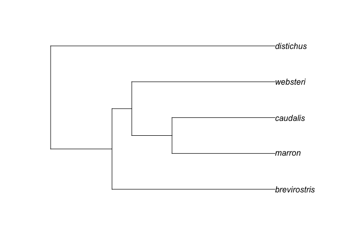
Some of the tests in ENMTools, including some really neat ones that are still in development, require you to build an enmtools.clade object. These objects are simply lists that contain a phylogeny and a set of enmtools.species objects. It's important that the names of the species objects and their species.name attributes match the names in the phylogeny's tip.labels. For demonstration, we're going to build an object for a clade of five anoles from Hispaniola. We have the tree, so we're just going to grab occurrence data from GBIF using the rgbif package.
library(rgbif)
library(ape)

##
## Attaching package: 'ape'

## The following objects are masked from 'package:raster':
##
##     rotate, zoom

hisp.anoles <- read.nexus(file = "test/testdata/StarBEAST_MCC.species.txt")

keepers <- c("brevirostris", "marron", "caudalis", "websteri", "distichus")

hisp.anoles <- drop.tip(phy = hisp.anoles, tip = hisp.anoles$tip.label[!hisp.anoles$tip.label %in% keepers])
plot(hisp.anoles)
So there's our tree. Now we're going to grab some environmental data.
hisp.env <- stack(list.files("test/testdata/Hispaniola_Worldclim", full.names = TRUE))
hisp.env <- setMinMax(hisp.env)
And then we'll create a function to build species from GBIF.
# Automate the process of downloading data and removing duds and dupes
species.from.gbif <- function(genus, species, name = NA, env){

  # Name it after the species epithet unless told otherwise
  if(is.na(name)){
    name <- species
  }

  # Get GBIF data
  this.sp <- enmtools.species(presence.points = gbif(genus = genus, species = species)[,c("lon", "lat")],
                              species.name = name)

  # Rename columns, get rid of duds
  colnames(this.sp$presence.points) <- c("Longitude", "Latitude")
  this.sp$presence.points <- this.sp$presence.points[complete.cases(extract(env, this.sp$presence.points)),]
  this.sp$presence.points <- this.sp$presence.points[!duplicated(this.sp$presence.points),]

  this.sp$range <- background.raster.buffer(this.sp$presence.points, 50000, mask = hisp.env)

  return(this.sp)
}
Now we'll create five species and add them to a species.clade object that is called brev.clade.
brevirostris <- species.from.gbif(genus = "Anolis", species = "brevirostris", env = hisp.env)
marron <- species.from.gbif(genus = "Anolis", species = "marron", env = hisp.env)
caudalis <- species.from.gbif(genus = "Anolis", species = "caudalis", env = hisp.env)
websteri <- species.from.gbif(genus = "Anolis", species = "websteri", env = hisp.env)
distichus <- species.from.gbif(genus = "Anolis", species = "distichus", env = hisp.env)


brev.clade <- enmtools.clade(species = list(brevirostris, marron, caudalis, websteri, distichus), tree = hisp.anoles)
check.clade(brev.clade)

##
##
## An enmtools.clade object with 5 species
##
## Species names:
##   brevirostris    caudalis    distichus   marron      websteri
##
## Tree:
##
## Phylogenetic tree with 5 tips and 4 internal nodes.
##
## Tip labels:
## [1] "brevirostris" "caudalis"     "distichus"    "marron"
## [5] "websteri"
##
## Rooted; includes branch lengths.
##
##
## Data Summary:
##
##
##                species.names   in.tree   presence   background   range
## -------------  --------------  --------  ---------  -----------  --------
## brevirostris   brevirostris    TRUE      173        0            present
## caudalis       caudalis        TRUE      21         0            present
## distichus      distichus       TRUE      678        0            present
## marron         marron          TRUE      12         0            present
## websteri       websteri        TRUE      17         0            present
That's one way to build a clade object by hand, but there's already one built into ENMTools to experiment with so we'll just use that.
data(iberolacerta.clade)
The AOC tests allow you to examine patterns of range, point, and ENM overlap in the context of a phylogeny. This is effectively a generalized version of several analyses: age-range correlation (e.g., Fitzpatrick and Turelli 2006), ENM overlap in the context of a phylogeny (e.g., Knouft et al. 2006, Warren et al. 2008), and point overlaps (e.g., Cardillo and Warren 2016).
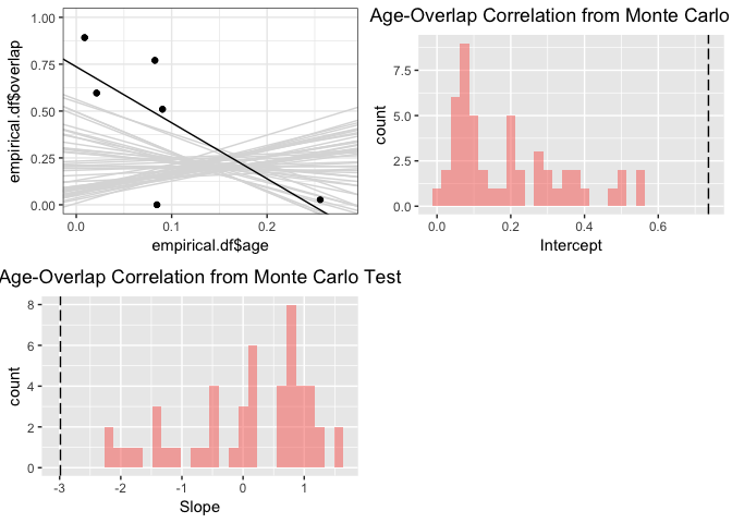
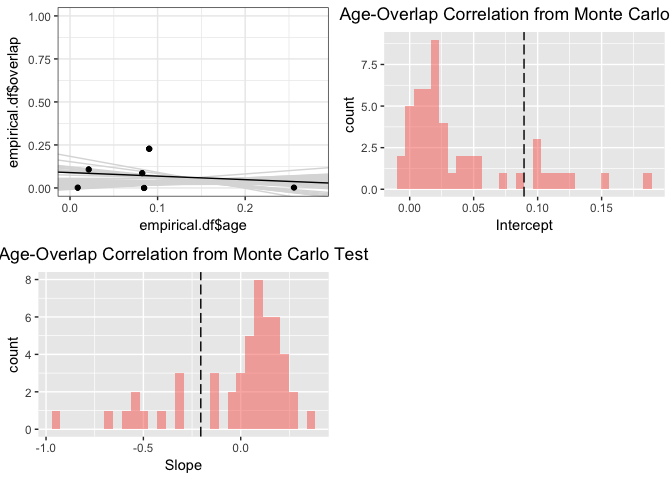
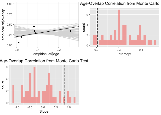
These tests require the creation of an enmtools.clade object, as above. AOC tests consist of two steps: first, the average overlap at each node in the phylogeny is calcualted using a method that takes tree topology into account (see Fitzpatrick and Turelli 2006), then we perform a linear regression to measure the relationship between node age and average overlap. Due to the fact that these overlaps violate many of the assumptions of a regular linear regression, however (e.g., errors are not iid), we can't calculate significance in the typical way. Instead we performa Monte Carlo test, permuting the identity of the tips of the tree and repeating the node averaging and modeling steps. Finally we measure statistical significance by comparing the empirical slope and intercept to the distribution of slopes and intercepts from the Monte Carlo replicates.
First, let's do one using geog.range.overlaps, as in Fitzpatrick and Turelli 2006. Note that this analysis requires that each of your species have a range raster stored in their species object (we did that as part of the function used above).
range.aoc <- enmtools.aoc(clade = iberolacerta.clade,  nreps = 50, overlap.source = "range")
summary(range.aoc)

##
##
## Age-Overlap Correlation test
##
## 50 replicates
##
## p values:
##      (Intercept) empirical.df$age
##       0.03921569       0.03921569

## `stat_bin()` using `bins = 30`. Pick better value with `binwidth`.
## `stat_bin()` using `bins = 30`. Pick better value with `binwidth`.
## NULL
Now we can do one using point overlaps just by changing the overlap.source argument:
point.aoc <- enmtools.aoc(clade = iberolacerta.clade,  nreps = 50, overlap.source = "points")
summary(point.aoc)

##
##
## Age-Overlap Correlation test
##
## 50 replicates
##
## p values:
##      (Intercept) empirical.df$age
##        0.3921569        0.4313725

## `stat_bin()` using `bins = 30`. Pick better value with `binwidth`.
## `stat_bin()` using `bins = 30`. Pick better value with `binwidth`.
## NULL
Or we can use similarity between ENMs built for each species. Here we'll use GLM models:
glm.aoc <- enmtools.aoc(clade = iberolacerta.clade,  env = env, nreps = 50, overlap.source = "glm", f = pres ~ poly(bio1, 2) + poly(bio12, 2))

##
##
## No background points provided, drawing background from range raster.
##
## Adding environmental data to species monticola
##  Processing presence points...
##  Processing background points...
##
##
## No background points provided, drawing background from range raster.
##
## Adding environmental data to species martinezricai
##  Processing presence points...
##  Processing background points...
##
##
## No background points provided, drawing background from range raster.
##
## Adding environmental data to species cyreni
##  Processing presence points...
##  Processing background points...
##
##
## No background points provided, drawing background from range raster.
##
## Adding environmental data to species horvathi
##  Processing presence points...
##  Processing background points...
##
##
## No background points provided, drawing background from range raster.
##
## Adding environmental data to species aurelioi
##  Processing presence points...
##  Processing background points...
##
##
## No background points provided, drawing background from range raster.
##
## Adding environmental data to species aranica
##  Processing presence points...
##  Processing background points...
##
##
## No background points provided, drawing background from range raster.
##
## Adding environmental data to species bonnali
##  Processing presence points...
##  Processing background points...

summary(glm.aoc)

##
##
## Age-Overlap Correlation test
##
## 50 replicates
##
## p values:
##      (Intercept) empirical.df$age
##        0.1960784        0.2352941

## `stat_bin()` using `bins = 30`. Pick better value with `binwidth`.
## `stat_bin()` using `bins = 30`. Pick better value with `binwidth`.
## NULL
*Broennimann, O., Fitzpatrick, M. C., Pearman, P. B., Petitpierre, B., Pellissier, L., Yoccoz, N. G., Thuiller, W., Fortin, M.-J., Randin, C., Zimmermann, N. E., Graham, C. H. and Guisan, A. (2012), Measuring ecological niche overlap from occurrence and spatial environmental data. Global Ecology and Biogeography, 21: 481–497. doi:10.1111/j.1466-8238.2011.00698.x*
Fitzpatrick, B. M., & Turelli, M. (2006). The geography of mammalian speciation: mixed signals from phylogenies and range maps. Evolution, 60(3), 601-615.
Knouft, J. H., Losos, J. B., Glor, R. E., & Kolbe, J. J. (2006). Phylogenetic analysis of the evolution of the niche in lizards of the Anolis sagrei group. Ecology, 87(sp7).
Levins, R. 1968. Evolution In Changing Environments. Monographs in Population Biology, volume 2. Princeton University Press, Princeton, New Jersey, USA.
Schoener, T. W. 1968. Anolis lizards of Bimini: resource partitioning in a complex fauna. Ecology 49:704- 726.
Warren, D.L., R.E. Glor, and M. Turelli. 2008. Environmental niche identity versus conservatism: quantitative approaches to niche evolution. Evolution 62:2868-2883. doi: 10.1111/j.1558-5646.2008.00482.x
Warren, D.L., M. Cardillo, D.F. Rosauer, and D.I. Bolnick. 2014. Mistaking geography for biology: inferring processes from species distributions. Trends in Ecology and Evolution 29 (10), 572-580. doi: 10.1016/j.tree.2014.08.003
