DifferentialDynamicProgramming

Installation

The package is registered and can be added with
] add DifferentialDynamicProgramming
The latest version is formally compatible with Julia v1.1+ (but probably works well for julia v1.0 as well if you dev it).

Demo functions

The following demo functions are provided

demo_linear() To run the iLQG DDP algorithm on a simple linear problem
demoQP To solve a demo quadratic program
demo_pendcart() Where a pendulum attached to a cart is simulated.

Usage

Demo linear

See demo file demo_linear.jl for a usage example.

# make stable linear dynamics
h = .01         # time step
n = 10          # state dimension
m = 2           # control dimension
A = randn(n,n)
A = A-A'        # skew-symmetric = pure imaginary eigenvalues
A = exp(h*A)    # discrete time
B = h*randn(n,m)

# quadratic costs
Q    = h*eye(n)
R    = .1*h*eye(m)

# control limits
lims = [] #ones(m,1)*[-1 1]*.6

T    = 1000             # horizon
x0   = ones(n,1)        # initial state
u0   = .1*randn(m,T)    # initial controls

# optimization problem
N    = T+1
fx   = A
fu   = B
cxx  = Q
cxu  = zeros(size(B))
cuu  = R

# Specify dynamics functions
function lin_dyn_df(x,u,Q,R)
    u[isnan(u)] = 0
    cx  = Q*x
    cu  = R*u
    fxx=fxu=fuu = []
    return fx,fu,fxx,fxu,fuu,cx,cu,cxx,cxu,cuu
end
function lin_dyn_f(x,u,A,B)
    u[isnan(u)] = 0
    xnew = A*x + B*u
    return xnew
end

function lin_dyn_cost(x,u,Q)
    c = 0.5*sum(x.*(Q*x)) + 0.5*sum(u.*(R*u))
    return c
end

f(x,u,i)     = lin_dyn_f(x,u,A,B,Q,R)
costfun(x,u) = lin_dyn_cost(x,u,Q)
df(x,u)      = lin_dyn_df(x,u,Q,R)

# run the optimization

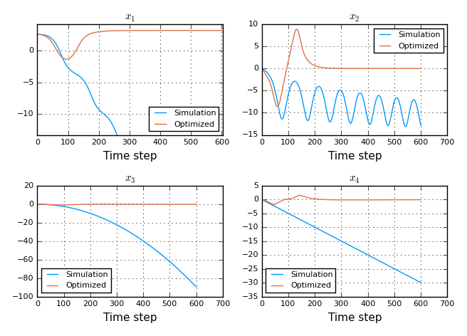
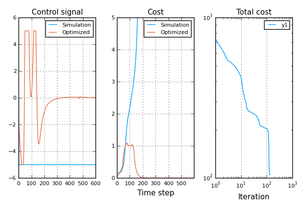
@time x, u, L, Vx, Vxx, cost, otrace = iLQG(f, costfun ,df, x0, u0, lims=lims);

Demo pendulum on cart

There is an additional demo function demo_pendcart(), where a pendulum attached to a cart is simulated. In this example, regular LQG control fails in stabilizing the pendulum at the upright position due to control limitations. The DDP-based optimization solves this by letting the pendulum fall, and increases the energy in the pendulum during the fall such that it will stay upright after one revolution.

Citing

This code consists of a port and extensions of a MATLAB library provided by the autors of

BIBTeX:
@INPROCEEDINGS{
  author    = {Tassa, Y. and Mansard, N. and Todorov, E.},
  booktitle = {Robotics and Automation (ICRA), 2014 IEEE International Conference on},
  title     = {Control-Limited Differential Dynamic Programming},
  year      = {2014}, month={May}, doi={10.1109/ICRA.2014.6907001}}
  http://www.mathworks.com/matlabcentral/fileexchange/52069-ilqg-ddp-trajectory-optimization
  http://www.cs.washington.edu/people/postdocs/tassa/

The code above was extended with KL-divergence constrained optimization for the thesis Bagge Carlson, F., "Machine Learning and System Identification for Estimation in Physical Systems" (PhD Thesis 2018).

@thesis{bagge2018,
  title        = {Machine Learning and System Identification for Estimation in Physical Systems},
  author       = {Bagge Carlson, Fredrik},
  keyword      = {Machine Learning,System Identification,Robotics,Spectral estimation,Calibration,State estimation},
  month        = {12},
  type         = {PhD Thesis},
  number       = {TFRT-1122},
  institution  = {Dept. Automatic Control, Lund University, Sweden},
  year         = {2018},
  url          = {https://lup.lub.lu.se/search/publication/ffb8dc85-ce12-4f75-8f2b-0881e492f6c0},
}