TestMechs

The TestMechs package implements the methodology from the paper “Testing Mechanisms” by Soonwoo Kwon and Jonathan Roth. The package provides tests for the “sharp null of full mediation”, which conjectures that the effect of a treatment operates through a particular conjectured mechanism (or set of mechanisms) M. It also provides lower bounds on the fraction of “always-takers” who are affected by the treatment despite having the same value of M regardless of treatment status. For now, the package assumes that the treatment is as good as randomly assigned (as in an RCT); we hope to add support for conditional random assignment in future iterations of the package. Note that the approach in the paper requires the mediator $M$ to be discrete.

Installation

You can install the development version of TestMechs from GitHub with:

# Install devtools if not already installed
install.packages("devtools")

# Install package
devtools::install_github("jonathandroth/TestMechs")

Application to Baranov et al. (2020)

We illustrate how the package can be used by walking through how the code can be applied to the application of Baranov et al. (2020) in Section 5.2 of “Testing Mechanisms”. In Baranov et al. (2020), $D$ is a treatment for depression and $Y$ is an index of outcomes for women’s financial empowerment. We are interested in whether the effect of $D$ on $Y$ can be explained by a mediator, or set of mediators, $M$. We consider three choices for $M$: (a) the presence of a grandmother in the home, (b)relationship quality with the woman’s husband, and (c) the combination of these two mechanisms.

We start with loading the required packages and the data.

# Load TestMechs
library(TestMechs)

# Load other packages that are required to run the example
library(dplyr)
library(ggplot2)
library(haven)

# Load data
data("baranov_data")

# Restrict to the experimental sample
mother_data <- mother_data %>% filter(THP_sample == 1)

We begin with the case where $M$ is a binary indicator for the presence of a grandmother in the home. The outcome variable $Y$ is continuous, and for ease of transparency and for conducting inference, we discretize the outcome into 5 bins based on the unconditional quantiles of the outcome. As noted in the paper, the test still remains valid under such a discretization but potentially loses sharpness. With some abuse of notation, we from now on write $Y$ to refer to this discretized outcome.

The main functions we will be using are: 1) partial_density_plot() to plot the partial densities to visually detect potential violations of the sharp null, 2) test_sharp_null() to conduct a statistical test for the sharp null and 3) lb_frac_affected() to compute the sharp lower bound for the fraction of always-takers (or never-takers) that are affected by treatment. While this example covers the basic usage of these functions, please refer to the documentation of each function (e.g., ?test_sharp_null) for a more detailed description.

Graphical Evidence

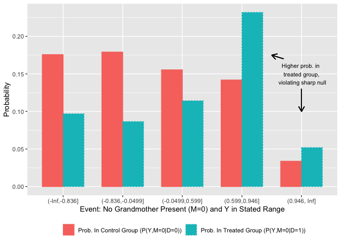
We first provide graphical evidence using a partial density plot using the function partial_density_plot(). When $M$ is binary, such (partial) density plots are often helpful to understand where the violations of the sharp null are coming from. The following snippet reproduces Figure 3 of the main paper.

nt_plot <-
  partial_density_plot(df = mother_data,
                       d = "treat",
                       m = "grandmother",
                       y = "motherfinancial",
                       num_Ybins = 5,
                       plot_nts = T,
                       density_1_label = "Prob. In Treated Group (P(Y,M=0|D=1))",
                       density_0_label = "Prob. In Control Group (P(Y,M=0|D=0))") +
  ylab("Probability") +
  xlab("Event: No Grandmother Present (M=0) and Y in Stated Range")

nt_plot +
  annotate(geom = "text", 
           x = 5,y=0.15,
           label = "Higher prob. in \n treated group, \n violating sharp null", size = 3) +
  geom_segment(x=4.7,y=0.17,
               xend = 4.5, yend = 0.175,
               arrow = arrow(length = unit(0.03,"npc")),
               color = "black", show.legend = F) +
  
  geom_segment(x=5,y=0.13,
               xend = 5, yend = 0.10,
               arrow = arrow(length = unit(0.03,"npc")),
               color = "black", show.legend = F) +  
  theme(legend.position="bottom",
        legend.title = element_blank())

This figure shows estimates of $P(Y=y,M=0 \mid D=d)$ for both $d=1$ and $d=0$. Under monotonicity, as shown in Section 2 of the paper, we should have that $P(Y=y, M=0 \mid D=1) \leq P(Y=y, M=0 \mid D=0)$ for all values of $y$. In other words, there should be a negative treatment effect on the compound outcome $1[Y=y,M=0]$ (i.e. have outcome $y$ and no grandmother present). As shown in the figure, however, this inequality appears to be violated at large values of $y$, suggesting that the outcome for some treated never-takers improved when receiving the treatment.

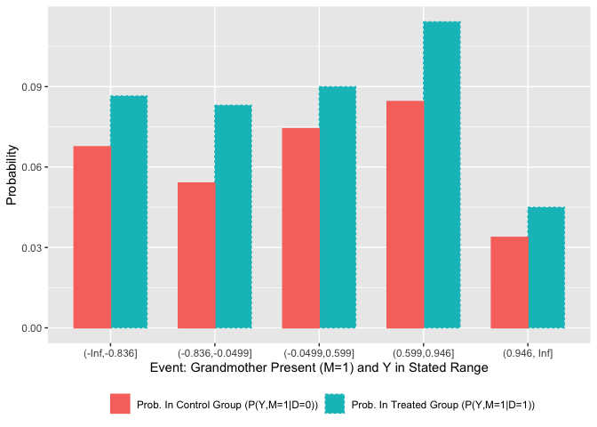
The argument plot_nts = T tells the package to make a plot showing the inequalities corresponding to there being no treatment effect for the “never-takers” (i.e. individuals with $M=0$ under both treatments). If instead plot_nts is set to F, we get a similar plot for the always-takers, which checks whether $P(Y=y, M=1 \mid D=1) \geq P(Y=y, M=1 \mid D=0)$. In this example, these inequalities appear to be satisfied, and so we cannot reject that there is no effect of the treatment on the always-takers.

at_plot <-
  partial_density_plot(df = mother_data,
                       d = "treat",
                       m = "grandmother",
                       y = "motherfinancial",
                       num_Ybins = 5,
                       plot_nts = F,
                       density_1_label = "Prob. In Treated Group (P(Y,M=1|D=1))",
                       density_0_label = "Prob. In Control Group (P(Y,M=1|D=0))") +
  ylab("Probability") +
  xlab("Event: Grandmother Present (M=1) and Y in Stated Range")

at_plot  +
  theme(legend.position="bottom",
        legend.title = element_blank())

Testing the sharp null of full mediation

While the figure above hints at a possible violation of the sharp null, it does not come with any uncertainty quantification. The function test_sharp_null() conducts statistical inference of the sharp null using the method described in Section 4 of the paper. The following snippet runs this test based on the test proposed in Cox and Shi (2023), which is our recommended approach for most applications. The package supports using the tests provided by Andrews, Roth, and Pakes (2023) and Fang, Santos, Shaikh, and Torgovitsky (2023); these methods can be specified by changing the method argument from "CS" to "ARP" or "FSST". When M is binary, as in our example here, one can also use the test from Kitagawa (2015) by setting method = "toru".

test_result <- test_sharp_null(df = mother_data,
                               d = "treat",
                               m = "grandmother",
                               y = "motherfinancial",
                               method = "CS", #use Cox and Shi test
                               num_Ybins = 5, #discretize using 5 bins
                               cluster = "uc") #cluster SEs at uc level
#> Loading required package: lpinfer

test_result$pval
#>            [,1]
#> [1,] 0.02283916

The test gives a p-value of 0.023, and thus the sharp null is rejected at the 5% significance level. Here, the p-value corresponds to the smallest value of $\alpha$ for which the test rejects. As mentioned above, we discretize the outcome variable to 5 bins as can be seen from the argument num_Ybins = 5. Currently, the function discretizes $Y$ into 5 bins if a num_Ybins value is not provided but $Y$ takes more than $30$ distinct values in the data. Because all of the methods rely on a central limit theorem approximation, one should choose the number of bins small enough such that the central limit theorem is reasonable within cells defined by the combination of $(Y,M,D)$.

Calculating the lower bound on fraction of always-takers affected by outcome

The test above suggests that the treatment effect does not operate entirely through the presence of a grandmother in the home. There are some people (never-takers) whose outcome is affected by the treatment despite having no change in $M$. It must be that some other mechanism mattered for these people. But how prevelant are these alternative mechanisms?To give a sense, we now compute lower bounds on the fraction of never-takers whose outcome is affected by the treatment despite having the same value of $M$ under both treatments. This gives a sense of the strength of mechanisms other than $M$: it tells us what fraction of the never-takers have a direct effect of the treatment. The definition of the lower bounds can be found in Section 3.1 of the paper. The function lb_frac_affected computes (a point estimate of) this lower bound. The argument at_group = 0 corresponds to computing this lower bound for the never-takers, who are referred to as “0-always takers” in the more general notation in the paper.

lb_nts <- lb_frac_affected(df = mother_data,
                           d = "treat",
                           m = "grandmother",
                           y = "motherfinancial",
                           num_Ybins = 5,
                           at_group = 0)
lb_nts
#> [1] 0.1858912

Our estimates of the lower bound imply that at least 19 percent of never-takers are affected by the treatment. One could likewise test the fraction of never-takers affected by setting at_group = 1 (in this case, the lower bound is zero). If at_group is set to NULL, then the package calculates the fraction pooling across all types that have the same value of $M$ under both treatments (i.e. always-takers and never-takers when $M$ is binary.)

Allowing for defiers

By default, TestMechs imposes the monotonicity assumption that the treatment can only increase the value of $M$. In this setting, this means that everyone who would have a grandmother present without receiving CBT treatment would also have one present when receiving CBT treatment. We can relax this assumption by setting the max_defiers_share parameter to be non-zero, which bounds the number of “defiers” by max_defiers_share.

We rerun the test above with max_defiers_share = .01, which allows one percent of the population to be defiers.

test_result_defiers <- test_sharp_null(df = mother_data,
                                       d = "treat",
                                       m = "grandmother",
                                       y = "motherfinancial",
                                       method = "CS",
                                       num_Ybins = 5,
                                       cluster = "uc",
                                       max_defiers_share = .01)

test_result_defiers$pval
#>            [,1]
#> [1,] 0.04630939

The p-value increases to 0.046, so the test rejects the sharp null even if you allow one percent of the population to be defiers. (Allowing for larger shares of defiers will eventually lead to an insignificant result.)

Likewise, we can also calculate the lower bound on the fraction of never-takers under this relaxed monotonicity.

lb_nts_defiers <- lb_frac_affected(df = mother_data,
                                   d = "treat",
                                   m = "grandmother",
                                   y = "motherfinancial",
                                   num_Ybins = 5,
                                   at_group = 0,
                                   max_defiers_share = .01)
lb_nts_defiers
#> [1] 0.1716415

Our estimates of the lower bound imply that at least 17 percent of never-takers are affected by the treatment when we allow one percent of the population to be defiers.

Results for an alternative mechanism (relationship quality with husband)

We next turn to the setting where we are interested in testing whether the effect is mediated by relationship quality with the husband, which is measured on a 1-5 scale. We can again test the sharp null and estimate a lower bound on the fraction affected.

test_sharp_null(df = mother_data,
                d = "treat",
                m = "relationship_husb",
                y = "motherfinancial",
                num_Ybins = 5,
                method = "CS",
                cluster = "uc")$pval
#>            [,1]
#> [1,] 0.02838332

Again, we reject the sharp null that all the treatment effect goes through the relationship quality with the husband.

We can also estimate a lower bound on the fraction of always-takers:

lb_frac_affected(df = mother_data,
                 d = "treat",
                 m = "relationship_husb",
                 y = "motherfinancial",
                 num_Ybins = 5,
                 at_group = NULL,
                 allow_min_defiers = TRUE)
#> [1] 0.1002207

Here, the parameter at_group = NULL asks the function compute the lower bound on the fraction of always-takers, pooled across different $M$ values, which it calculates to be around 10 percent. (The empirical distribution suggests a small violation of monotonicity, although it is not statistically significant; the argument allow_min_defiers = TRUE calculates the lower bound allowing for the minimum number of defiers consistent with the empirical distribution — see footnote 25 of the paper for details.)

We note that while the method works with multi-valued discrete mediators (such as our 1-5 score), we generally expect the power of the test to decrease as one approaches an approximately continuous mediator. See the discussion in Remarks 2 and 3 of the paper regarding power and discretization of $M$.

Combination of both mechanisms

Finally, we test the null hypothesis that the treatment effect is explained by the combination of the two mechanisms. This is done by passing a vector of variables names for the m argument.

test_result_both <- test_sharp_null(df = mother_data,
                                    d = "treat",
                                    m = c("relationship_husb",
                                          "grandmother"),
                                    y = "motherfinancial",
                                    num_Ybins = 5,
                                    method = "CS",
                                    cluster = "uc")

test_result_both$pval
#>           [,1]
#> [1,] 0.6540865

With a p-value of 0.654, we cannot reject the sharp null that the combination of presence of grandmother and relationship quality with husband fully explain the treatment effect.

Again, we can estimate a lower bound on the fraction of those affected by treatment, pooled across different $M$ values:

lb_frac_both <- lb_frac_affected(df = mother_data,
                                 d = "treat",
                                 m = c("relationship_husb",
                                       "grandmother"),
                                 y = "motherfinancial",
                                 num_Ybins = 5,
                                 allow_min_defiers = TRUE)
lb_frac_both
#> [1] 0.07251284

We estimate a lower bound of 7 percent, although this does not appear to be statistically significant given the test result above.