The pretrends package provides tools for power calculations for
pre-trends tests, and visualization of possible violations of parallel
trends. Calculations are based on Roth (2022).
This is the Stata version of the R package of the same name.
(Please cite the paper if you enjoy the package!)
The basic idea is that if we are relying on a pre-trends test to verify the parallel trends assumption, we’d like that test to have power to detect relevant violations of parallel trends. To assess the power of a pre-trends test, we can calculate its ex ante power: how big would a violation of parallel trends need to be such that we would detect it some specified fraction (say 80%) of the time? This is similar to the minimal detectable effect (MDE) size commonly reported for RCTs. Alternatively, we can calculate how likely we would be to detect a particular hypothesized violation of parallel trends. The pretrends package provides methods for doing these calculations, as well as for visualizing potential violations of parallel trends on an event-study plot.
If you’re worried about violations of parallel trends, you might also consider the sensitivity analysis provided in the HonestDiD package. Rather than relying on the significance of a pre-test, the HonestDiD approach imposes that the post-treatment violations of parallel trends are not “too large” relative to the pre-treatment violations. It then forms confidence intervals for the treatment effect that take into account the uncertainty over how big the pre-treatment violations of parallel trends are. (This, in my view, is a more “complete” solution to the issue that pre-trends tests may fail to detect violations of parallel trends.)
If you’re not an R or Stata user, you may also be interested in the associated Shiny app.
version 0.4.4 04Apr2024 | Installation | Application
The package may be installed by using net install:
local github https://raw.githubusercontent.com
net install pretrends, from(`github'/mcaceresb/stata-pretrends/main) replace
You can also clone or download the code manually, e.g. to
stata-pretrends-main, and install from a local folder:
cap noi net uninstall pretrends
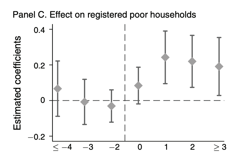
net install pretrends, from(`c(pwd)'/stata-pretrends-main)We illustrate how to use the package with an application to He and Wang (2017). The analysis will be based on the event-study in Figure 2C, which looks like this:
We first load the dataset used by He and Wang.
use "https://media.githubusercontent.com/media/mcaceresb/stata-pretrends/main/data/workfile_AEJ.dta", clearWe then run their regression specification.
reghdfe l_poor_reg_rate Lead_D4_plus Lead_D3 Lead_D2 D0 Lag_D1 Lag_D2 Lag_D3_plus, absorb(v_id year) cluster(v_id) dof(none)which yields the following results
             |               Robust
l_poor_reg~e |      Coef.   Std. Err.      t    P>|t|     [95% Conf. Interval]
-------------+----------------------------------------------------------------
Lead_D4_plus |   .0667032   .0943746     0.71   0.480    -.1191533    .2525596
     Lead_D3 |  -.0077018   .0770514    -0.10   0.920    -.1594428    .1440392
     Lead_D2 |  -.0307691   .0551237    -0.56   0.577    -.1393268    .0777887
          D0 |   .0840307   .0626478     1.34   0.181    -.0393445    .2074059
      Lag_D1 |   .2424418   .0898103     2.70   0.007     .0655741    .4193096
      Lag_D2 |    .219879   .0887783     2.48   0.014     .0450438    .3947142
 Lag_D3_plus |   .1910925   .0989365     1.93   0.055    -.0037478    .3859329
       _cons |   1.478639   .0811732    18.22   0.000      1.31878    1.638497
To use the pretrends package, we need the results of an event-study, namely
the vector of event-study coefficients (beta), their variance-covariance
matrix (sigma), and the relative time periods they correspond to (t). For
this example, we use the beta and sigma saved from a two-way fixed effects
regression, but the pretrends package can accommodate an event-study from any
asymptotically normal estimator, including
Callaway and Sant’Anna (2020)
and Sun and Abraham (2020), so long as the resulting estimates and coefficients are saved in e(b) and e(V). If using a command that does not export an e(b) and e(V), instead provide the coefficients and covariance matrix directly via the beta() and vcov() options.
Using beta and sigma for this pretrends package is the same as for the HonestDiD package; see the HonestDiD package README for examples, including Callaway and Sant’Anna.
The package has two subcommands:
-
The
powersub-command calculates the slope of a linear violation of parallel trends that a pre-trends test would detect a specified fraction of the time. (By detect, we mean that there is any significant pre-treatment coefficient.) -
Alternatively, the user can specify a hypothesized violations of parallel trends—the package then creates a plot to visualize the results, and reports various statistics related to the hypothesized difference in trend. The user can specify a hypothesized linear pre-trend via the
slope()option, or provide an arbitrary violation of parallel trends via thedelta()option.
Let's illustrate the first use case:
pretrends power 0.5, pre(1/3) post(4/7)
* Slope for 50% power =  .0520662

return list
* scalars:
*               r(slope) =  .0520662479737356
*               r(Power) =  .5
In the command above, the option pre(1/3) tells the package that the
pre-treatment event-study coefficients are in positions 1 through 3 in
our regression results. (The package assumes that the period before the
event-study is normalized to zero and omitted from the regression.) Likewise,
the option post(4/7) tells the package that the post-treatment coefficients
are in positions 4 through 7.
The results tell us that if there were a linear pre-trend with a slope
of about 0.05, then we would find a significant pre-trend only half the
time. (Note that the result of the pretrends power subcommand is a
magnitude, and thus is always positive.) If we want wanted a different power
threshold, say 80%, we would change power 0.5 to power 0.8 in the command
above.
The package’s second function enables power analyses and visualization given the results of an event-study and a user-hypothesized violation of parallel trends. We illustrate this using the linear trend against which pre-tests have 50 percent power, computed above. (This is just for illustration; we encourage researchers to conduct power analysis for violations of parallel trends they deem to be relevant in their context.) We run the command:
matrix sigma = e(V)
matrix beta  = e(b)
matrix beta  = beta[., 1..7]
matrix sigma = sigma[1..7, 1..7]
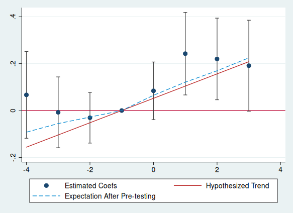
pretrends, numpre(3) b(beta) v(sigma) slope(`r(slope)')
The command tells Stata to visualize a linear violation of parallel trends with a given slope. Heuristically, the event-plot is more convincing if an economically plausible violation of parallel trends cannot explain the pattern in the event-study (e.g. go through all of the confidence intervals); see the HonestDiD package for a formalization of this idea.
In the example above, r(slope) conains 0.052. If instead you wanted
to visualize a linear violation with slope 5, you'd just specify
slope(5). (Note when specifying numpre() the vector b() and the
matrix v() must only contain the relevant coefficients.) The resulting
plot super-imposes the conjectured linear violation of parallel trends on
the event-plot in red. It also shows in dashed blue what we'd expect the
coefficients to look like on average conditional on not finding a significant pre-trend
if in fact that truth was the hypothesized red line.
Note that to create the plot above, the coefplot package is required; if the
coefplot package is not installed or not available, the user can add option
nocoefplot to skip the visualization. In either case the event study data
is saved in r(), along several useful statistics about the power of the
pre-test against the hypothesized trend.
return list
* scalars:
*                  r(LR) =  .1057053251022486
*               r(Bayes) =  .5690176868657247
*               r(Power) =  .5000000000010107
*               r(slope) =  .0520662479737356
*
* macros:
*    r(PreTrendsResults) : "PreTrendsResults"
*
* matrices:
*             r(results) :  8 x 6
*               r(delta) :  1 x 8

* data for visualization
matlist r(results)
*              |         t    betahat         lb         ub  deltatrue  meanAft~g
* -------------+------------------------------------------------------------------
*           r1 |        -4   .0667032  -.1182677    .251674  -.1561987  -.0923171
*           r2 |        -3  -.0077018  -.1587197   .1433162  -.1041325  -.0555576
*           r3 |        -2  -.0307691  -.1388096   .0772715  -.0520662  -.0279117
*           r4 |        -1          0          0          0          0          0
*           r5 |         0   .0840307  -.0387567    .206818   .0520662   .0649147
*           r6 |         1   .2424418   .0664168   .4184668   .1041325   .1208691
*           r7 |         2    .219879   .0458768   .3938812   .1561987   .1694932
*           r8 |         3   .1910925  -.0028194   .3850045    .208265   .2245753
An explanation of the returned results is as follows:
-
r(Power) The probability that we would find a significant pre-trend under the hypothesized pre-trend. (This is 0.50, up to numerical precision error, by construction in our example.) Higher power indicates that we would be likely to find a significant pre-treatment coefficient under the hypothesized trend.
-
r(BF) (Bayes Factor) The ratio of the probability of “passing” the pre-test under the hypothesized trend relative to under parallel trends. The smaller the Bayes factor, the more we should update our prior in favor of parallel trends holding (relative to the hypothesized trend) if we observe an insignificant pre-trend.
-
r(LR) (Likelihood Ratio) The ratio of the likelihood of the observed coefficients under the hypothesized trend relative to under parallel trends. If this is small, then observing the event-study coefficient seen in the data is much more likely under parallel trends than under the hypothesized trend.
-
r(results) The data used to make the event plot. Note the column
meanAfterPretesting, which is also plotted. The basic idea of this column is that if we only analyze our event-study conditional on not finding a significant pre-trend, we are analyzing a selected subset of the data. The meanAfterPretesting column tells us what we’d expect the coefficients to look like conditional on not finding a significant pre-trend if in fact the true pre-trend were the hypothesized trend specified by the researcher.
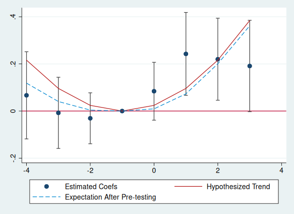
Last, although our example has focused on a linear violation of parallel trends, the package allows the user to input an arbitrary non-linear hypothesized trend. For instance, here is the event-plot and power analysis from a quadratic trend.
mata st_matrix("deltaquad", 0.024 * ((-4::3) :- (-1)):^2)
pretrends, time(-4(1)3) ref(-1) deltatrue(deltaquad) coefplot
return list
* scalars:
* r(LR) = .4332635420562206
* r(Bayes) = .3841447062350103
* r(Power) = .6624492391878117
* r(slope) = .
*
* macros:
* r(PreTrendsResults) : "PreTrendsResults"
*
* matrices:
* r(results) : 8 x 6
* r(delta) : 1 x 8
matlist r(results)
* | t betahat lb ub deltatrue meanAft~g
* -------------+------------------------------------------------------------------
* r1 | -4 .0667032 -.1182677 .251674 -.1561987 -.0923171
* r2 | -3 -.0077018 -.1587197 .1433162 -.1041325 -.0555576
* r3 | -2 -.0307691 -.1388096 .0772715 -.0520662 -.0279117
* r4 | -1 0 0 0 0 0
* r5 | 0 .0840307 -.0387567 .206818 .0520662 .0649147
* r6 | 1 .2424418 .0664168 .4184668 .1041325 .1208691
* r7 | 2 .219879 .0458768 .3938812 .1561987 .1694932
* r8 | 3 .1910925 -.0028194 .3850045 .208265 .2245753 (Note when specifying time() and ref()' by default the vector b() and the matrix v() must start with the relevant coefficients. The number of pre-period is taken to be the number of entries in the time vector strictly smaller than ref(), and the number of post-periods the number of entries strictly larger. time() and ref() may be combined with pre() and post(); numpre() may not be combined with either.)


