Summary

This project aims to share the current state and location of Brazilian Graduating Programs in Computer Science and related areas. The purpose is to realize an exploratory analysis of available data about Computing Programs and generate meaningful visualizations.

First Part

We will be based on this document made by CAPES, the Brazilian organization responsible for Higher Education Programs evaluation. Our attempt is to extract the needed information from this pdf file to perform our analysis. The information that we need is in pages 29-31. The first thing to do is to install and load the needed packages. In Ubuntu you may need to install libcurl4 and libcurl4-openssl-dev before installing pdftools and gdal-bin, proj-bin, libgdal-dev and libproj-dev before installing rgdal. You will also need to install gifski package to create the gifs with gganimate package. (libssl in ubuntu, libudunits2-dev)

if (!require(pdftools)) install.packages("pdftools", repos = "http://cran.us.r-project.org")
require(pdftools)

if (!require(dplyr)) install.packages("dplyr", repos = "http://cran.us.r-project.org")
  require(dplyr)

if (!require(readr)) install.packages("readr", repos = "http://cran.us.r-project.org")
require(readr)

if (!require(stringi)) install.packages("stringi", repos = "http://cran.us.r-project.org")
require(stringi)

if (!require(stringr)) install.packages("stringr", repos = "http://cran.us.r-project.org")
require(stringr)

if (!require(xlsx)) install.packages("xlsx", repos = "http://cran.us.r-project.org")
require(xlsx)

if (!require(rgdal)) install.packages("rgdal", repos = "http://cran.us.r-project.org")
require(rgdal)

if (!require(ggplot2)) install.packages("ggplot2", repos = "http://cran.us.r-project.org")
require(ggplot2)

if(!require(RColorBrewer)) install.packages("RColorBrewer", repos = "http://cran.us.r-project.org")
require(RColorBrewer)

if(!require(viridis)) install.packages("viridis", repos = "http://cran.us.r-project.org")
require(viridis)

if(!require(gganimate)) install.packages("gganimate", repos = "http://cran.us.r-project.org")
require(gganimate)

if(!require(ggrepel)) install.packages("ggrepel", repos = "http://cran.us.r-project.org")
require(ggrepel)

if(!require(gpclib)) install.packages("gpclib")
require(gpclib)

if(!require(maptools)) install.packages("maptools")
require(maptools)

gpclibPermit()

if(!require(mapproj)) install.packages("mapproj")
require(mapproj)

if(!require(gifski)) install.packages("gifski")
require(gifski)

if(!require(png)) install.packages("png")
require(png)

if(!require(av)) install.packages("av")
require(av)

if(!require(openssl)) install.packages("openssl")
require(openssl)

We load the data by lines using pdf_text and read_lines, select only the data of pages 29-31 (checking the file_pdf variable and selecting specific lines 1098:1190) and eliminate some lines with grep function using header words like "Coordenação" and "Diretoria", meaning that the line has not useful information about the programs.

file_pdf <- pdf_text("pdf/Evaluation report - Computer science.pdf") %>% read_lines()
file_pdf <- file_pdf[1098:1190]
file_pdf <- file_pdf[-(grep("Coordenação", file_pdf))]
file_pdf <- file_pdf[-(grep("Diretoria", file_pdf))]

There were some lines that were not properly read (because of information format), so it was easier to remove them. Of course, after we need to include them manually.

file_pdf <- file_pdf[-(24:28)] #Remove UFBA-UNIFACS-UEFS 
file_pdf <- file_pdf[-(34:35)]
file_pdf <- file_pdf[-(75:76)]
file_pdf <- file_pdf[-(44:46)] #Remove UFSCAR-Sorocaba
file_pdf <- file_pdf[-(47:49)] #Remove USP-ICMC

Useless information in some lines were changed to an empty string using gsub and after we split all data using spaces as the spliting criteria (by lines) through strsplit command.

file_pdf[56]<-gsub("-CA-MP","  ",file_pdf[56]) 
file_pdf[57]<-gsub("-IN-MP","  ",file_pdf[57]) 
file_pdf <- strsplit(file_pdf, "  ")

Now we use the following loop to remove the empty spaces generated above. The result is stored in list_pdf.

list_pdf <- 0
a <- 1
for(i in 1:length(file_pdf)){
    info_number <- length(file_pdf[[i]][!stri_isempty(file_pdf[[i]])])
    for(j in 1:info_number){
        list_pdf[a] <- str_trim(file_pdf[[i]][!stri_isempty(file_pdf[[i]])][j])
        a <- a + 1
    }
}

Now we create a new dataframe with the columns we want with data.frame command, initializing them with zeros. The loop catches every data needed by feature and stores in the new dataframe.

data_pdf <- data.frame(stringsAsFactors = FALSE, "Universidade" = 0, "Curso" = 0, "Nivel" = 0, "Nota" = 0)
a <- 1
for(i in seq(from = 2, to = length(list_pdf), by = 5)){
    data_pdf[a,1] <- list_pdf[i]
    data_pdf[a,2] <- list_pdf[i+1]
    data_pdf[a,3] <- list_pdf[i+2]
    data_pdf[a,4] <- list_pdf[i+3]
    a <- a + 1
}

Finally, we save this data into a xlsx file with write.xlsx command. Here we end the first part.

write.xlsx(data_pdf, file = "csv/universities_before.xlsx", col.names = TRUE, row.names = TRUE, append = FALSE)

NOTE: To verify if all Computer Graduating Programs were included, we checked the Sucupira Website. There, we verified that 11 Programs were missing, so we manually inserted them and also included the foundation year, latitude/longitude and city id. The city id was got from here, where we got the Brazilian states and cities information. The shapefile that we will use was got from here. You can get from here too. We also included the research topics of each one of the programs. To do that we went to each website of each program and registered each research topic. The structure of all extracted and collected data is divided in the following files:

universities_before.xlsx: contains information by university before the integration with Sucupira data.
universities_after.xlsx: contains information by university (id, university name, university code, course, program level, concept, latitude, longitude, city id and foundation year)
brazilian_cities.xlsx: contains all Brazilian cities, with state id to identify the state.
brazilian_states.xlsx: contains all Brazilian states, with state id to be used with brazilian_cities.xlsx.
research_names.xlsx: contains all research topics with an id to be used with the university_research.xlsx.
university_research.xlsx: the join between universities and their research topics.
graduation_level.xlsx: identifies the level of each Program: 0 to professional Master degree, 1 to academic Master degree, 2 to Doctoral/PhD degree and 3 to both Master and Doctoral degree.
course_name.xlsx: the names of graduation courses.
concentration_area: the concentration area of graduating programs.
university_concentration_area.xlsx: join between the graduating programs and its concentration area.

Second Part

Now, we have all data needed to perform our analysis. First, we load the needed data and check how they are organized.

universities <- read.xlsx("csv/universities_after.xlsx", sheetIndex = 1, encoding = "UTF-8")
brazilian_cities <- read.csv("csv/brazilian_cities.csv", sep = ",", stringsAsFactors = FALSE, encoding = "UTF-8")
brazilian_states <- read.csv("csv/brazilian_states.csv",sep = ",", stringsAsFactors = FALSE, encoding = "UTF-8")
research_names <- read.xlsx("csv/research_names.xlsx", sheetIndex = 1, encoding = "UTF-8")
university_research <- read.xlsx("csv/university_research.xlsx", sheetIndex = 1, encoding = "UTF-8")
graduation_level <- read.xlsx("csv/graduation_level.xlsx", sheetIndex = 1, encoding = "UTF-8")
course_name <- read.xlsx("csv/course_name.xlsx", sheetIndex = 1, encoding = "UTF-8")
concentration_area <- read.xlsx("csv/concentration_area.xlsx", sheetIndex = 1, encoding = "UTF-8")
university_concentration_area <- read.xlsx("csv/university_concentration_area.xlsx", sheetIndex = 1, encoding = "UTF-8")
shape_brazil <- readOGR("shapefile/Brazil.shp", "Brazil", use_iconv = TRUE)

Now we join the data from all excel files to a single dataframe, using left_join function.

all_data <- universities %>% left_join(brazilian_cities, by = c("city_id" = "ibge_code"))
all_data <- all_data %>% left_join(brazilian_states, by = c("state_id" = "state_id"))
all_data <- all_data %>% left_join(university_research, by = c("id" = "university_id"))
all_data <- all_data %>% left_join(research_names, by = c("research_id" = "id"))
all_data <- all_data %>% left_join(graduation_level, by = c("level" = "id"))
all_data <- all_data %>% left_join(course_name, by = c("course" = "id"))
all_data <- all_data %>% left_join(university_concentration_area, by = c("id" = "university_id"))
all_data <- all_data %>% left_join(concentration_area, by = c("concentration_area_id" = "id"))

From now on we will not use the ids, so we removed them too. We also convert the lat/long and grade data to numeric format.

all_data <- all_data[,-9]
all_data <- all_data[,-13]
all_data <- all_data[,-13]
all_data <- all_data[,-15]

all_data$latitude <- as.numeric(as.character(all_data$latitude))
all_data$longitude <- as.numeric(as.character(all_data$longitude))
all_data$grade <- as.numeric(as.character(all_data$grade))

To reuse some code, we save the theme and lab parameters in a variable.

theme <- theme(axis.text = element_text(size = 16),
              plot.caption = element_text(size = 12, face = "bold"),
              axis.title = element_text(size = 18, face = "bold"),
              legend.title = element_text(size = 18), 
              legend.text = element_text(size = 14),
              legend.key.size = unit(1.0, "cm"),
              legend.key.width = unit(0.4,"cm"),
              text = element_text(color = "#22211d"), 
              legend.background = element_rect(fill = "#dddddd", color = "black"),
              panel.background = element_rect(fill = "#BFD5E3", colour = "#6D9EC1"),
              plot.title = element_text(size = 22, hjust = 0.5, color = "#4e4d47"))

labs <- labs(x = "Longitude", y = "Latitude", caption = "Data source: Computer Science Graduating Programs - Sucupira Website")

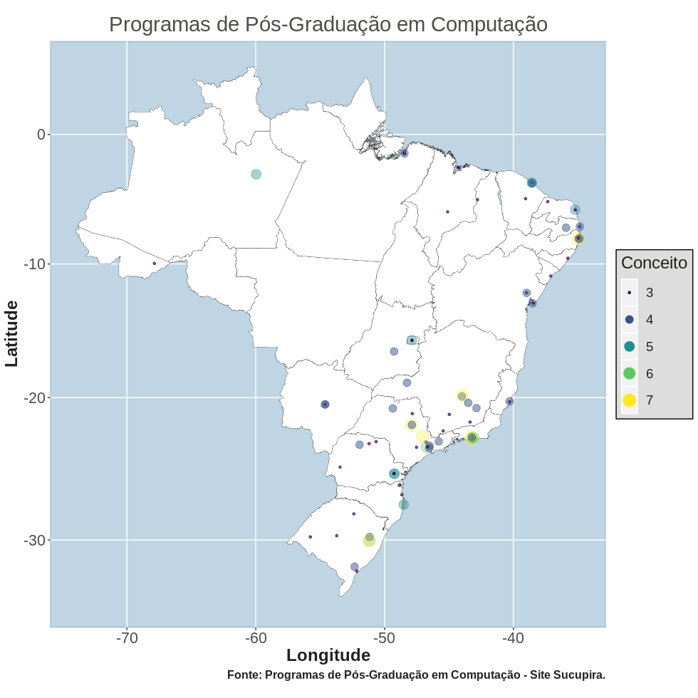
To generate the map below, we will use ggplot and some other functions. Let's understand the logic behind it.

1.   mybreaks <- as.numeric(c(3, 4, 5, 6, 7)) 
2.   ggplot() + 
3.   geom_polygon( data = shape_brazil, aes(x = long, y = lat, group = group), fill = "white", size = 0.1, color = "black") +
4.   geom_point( data = all_data[!duplicated(all_data$id),], aes(x = longitude, y = latitude, size = grade, color = grade, alpha = I(2/(grade)))) +
5.   scale_color_viridis(name = "Conceito", breaks = mybreaks) +
6.   scale_size_continuous(name = "Conceito", breaks = mybreaks) +
7.   coord_map() + 
8.   guides( colour = guide_legend(), alpha = FALSE) +
9.   ggtitle("Programas de Pós-Graduação em Computação") +
10.  labs(x = "Longitude", y = "Latitude") +
11.  theme + labs

Line 1: mybreaks is a variable to be used to assign all possible values to the legend.

Line 2: main ggplot function to generate graphics.

Line 3: geom_polygon is used to plot the map. Inside of aes we use all aesthetics we need to the polygons. We use shape as data (outside of aes), longitude as x-axis, latitude as y-axis and group as the group (generated variable when we transformed shapefile to dataframe, to group the information). fill argument is used to coloring, size argument is the size of polygons, and color for polygons.

Line 4: geom_point is used to plot points in the map. The data argument is the dataframe with data from Computing Graduating Courses. Aes argument: x-axis receives the longitude and y-axis receives the latitude from universities. The size argument is about the point size for each sample. The color argument is about the point color for each sample. The alpha argument is for the transparency of each data point. These three previous arguments will be proportional to the "Grade", a sinthetized value that represent (or should be) the quality of Brazilian Graduating Programs.

Line 5: scale_color_viridis is used to set what colors to use in the points. We give a name to be used in the legend and what are the possible values in the breaks argument, giving the value of mybreaks.

Line 6: scale_size_continuous is used to set the size of the points. We give a name to be used in the legend and what are the possible values in the breaks argument, giving the value of mybreaks.

Line 7: coord_map is used to preserve the real proportions of latitude and longitude.

Line 8: guides is used to set all the scales in the legend. In our case, we set the color scale using guide_legend in the colour argument. We do not want to use the alpha, so we set alpha to FALSE.

Line 9: ggtitle is used to set title to the whole plot.

Line 10: labs is used to set x-axis legend (x argument) and y-axis legend (y argument).

Line 11: theme is used to customize other graphical elements, including legends, background, panels and others. These values were previously set, like labs parameter, to customize the x-axis, y-axis and caption.

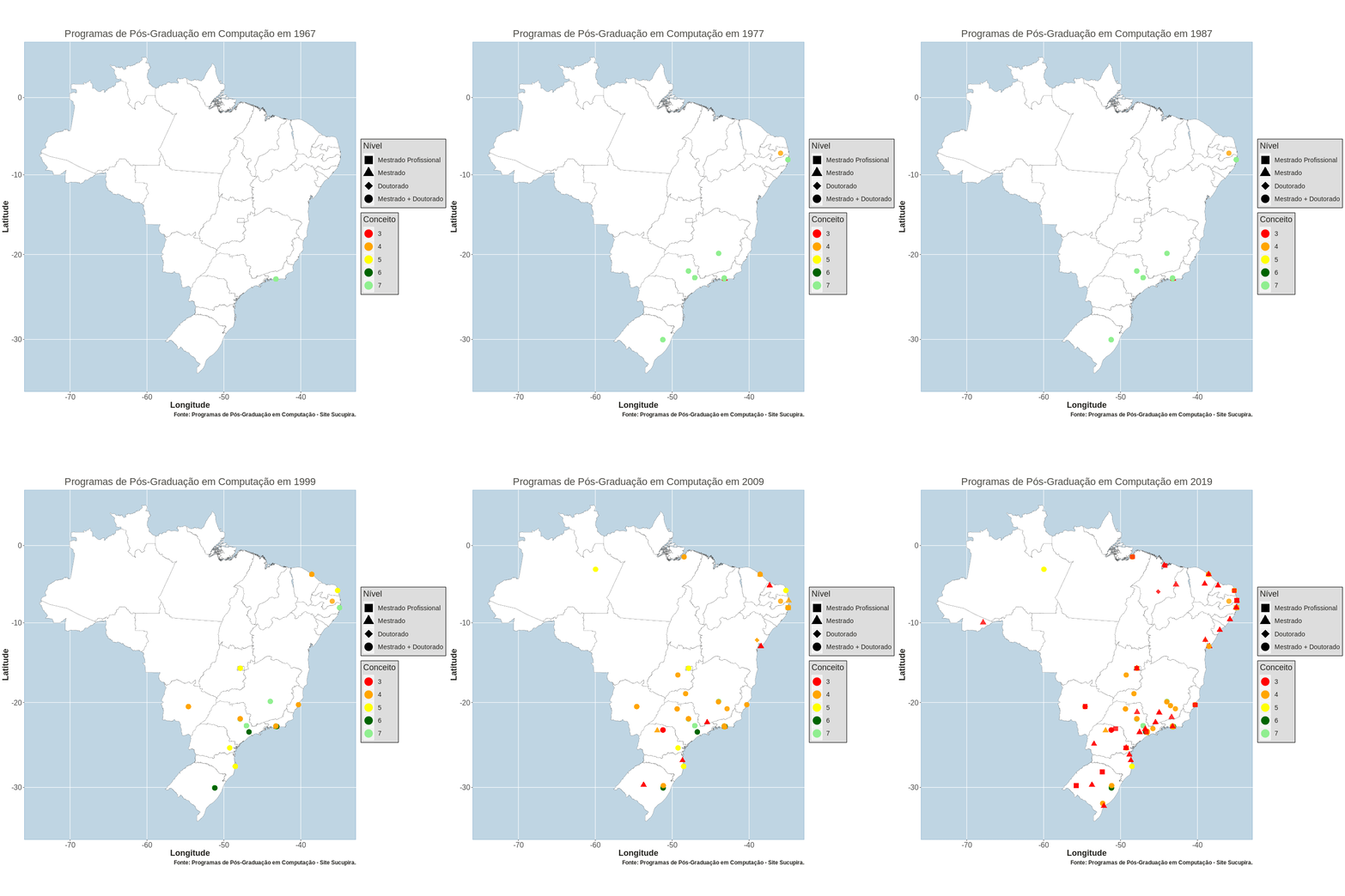
Now we create a gif using animate. We first get the values from level colunm and add 14 to match with values of shapes we want to plot after. shadow_mark with past argument is used to ensure that the points generated by previous frames continue in the plot. The frame_time in ggtitle is used to plot each different year in the title when the frame is changed. Transition_time is what argument we will use to separate each frame.

all_data$shape <- all_data$level + 14

p <- ggplot(data = all_data, aes(group = year)) +
     geom_polygon(data = shape_brazil, aes( x = long, y = lat, group = group), fill = "white", size = 0.1, color = "black") +
     geom_point(data = all_data, aes(x = longitude, y = latitude,  size = 4, color = as.factor(grade), alpha = 0.05,  group = year, shape = as.factor(shape))) +
     scale_color_manual(name = "Conceito", breaks = mybreaks, values = c("red","orange","yellow","dark green","light green")) +
     scale_shape_manual(name = "Nível", values = c(15, 17, 18, 19), labels = c("Mestrado Profissional","Mestrado","Doutorado","Mestrado + Doutorado")) +
     coord_map() +
     shadow_mark(past = TRUE) +
     guides(colour = guide_legend(override.aes = list(size = 8)), shape = guide_legend(override.aes = list(size = 8)), alpha = FALSE, size = FALSE) +
     ggtitle("Programas de Pós-Graduação em Computação em {round(frame_time,0)}") +
     transition_time(year) +
     theme + labs

animate(p, nframes = 52, fps = 1, width = 1800, height = 900, renderer = gifski_renderer("images/figure2.gif", loop = FALSE)) + ease_aes('cubic-in-out')

If you want to generate video instead of gifs, you can use the animate function below with ffmpeg_renderer. Note: you need first to download and install the ffmpeg in your system.

animate(p, nframes = 56, fps = 2, width = 1800, height = 900, renderer = ffmpeg_renderer()) + ease_aes('cubic-in-out')

We can also use the script below to generate an .avi video instead of gifs or ffmpeg renderer.

animate(p, width = 1800, nframes = 52, fps = 2, height = 1200, renderer = av_renderer('animation.mp4'))

Below some other examples.

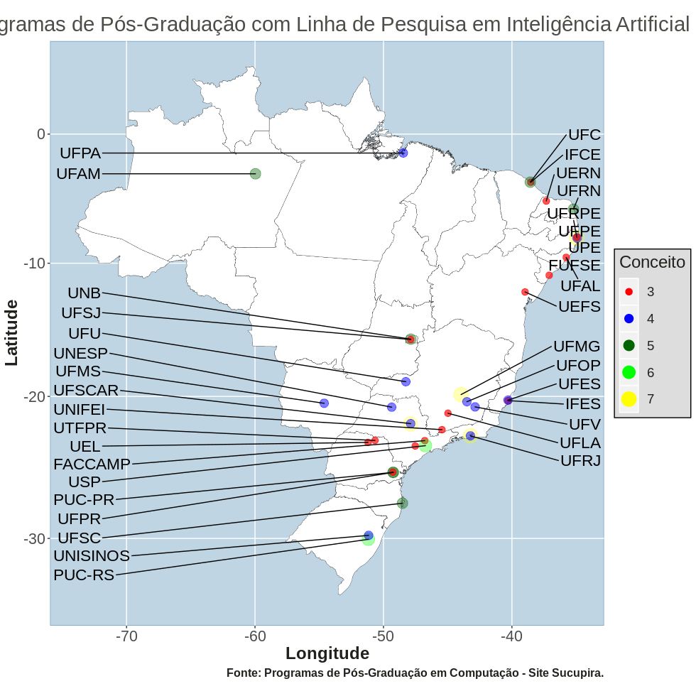
Brazilian Computer Graduating Programs that have Artificial Intelligence as a research line.

all_data_2 <- subset(all_data, all_data$research_name=="Inteligencia Artificial")

ggplot() + 
geom_polygon(data = shape_brazil, aes(x = long, y = lat, group = group), fill = "white", size = 0.1, color = "black") +
geom_point(data = all_data_2[!duplicated(all_data_2$id),], aes(x = longitude, y = latitude, size = as.factor(grade), color = as.factor(grade), alpha = I(2/grade))) +
scale_colour_manual(name = "Conceito", values = c("red","blue","dark green","green","yellow")) +
scale_size_manual(name = "Conceito", values = mybreaks) +
geom_text_repel(data = all_data_2[all_data_2$longitude > -45 & !duplicated(all_data_2$code),], aes(x = longitude, y = latitude, label = code, size = as.factor(6)), hjust = 0, nudge_x = -34 - subset(all_data_2, all_data_2$longitude > -45 & !duplicated(all_data_2$code))$longitude, direction = "y", show.legend = FALSE) +
geom_text_repel(data = all_data_2[all_data_2$longitude <= -45 & !duplicated(all_data_2$code),], aes(x = longitude, y = latitude, label = code, size = as.factor(6)), hjust = 1, nudge_x = -72 - subset(all_data_2, all_data_2$longitude <= -45 & !duplicated(all_data_2$code))$longitude, direction = "y", show.legend = FALSE) + 
coord_map() + 
guides() +
ggtitle("Programas de Pós-Graduação com Linha de Pesquisa em Inteligência Artificial") +
labs + theme

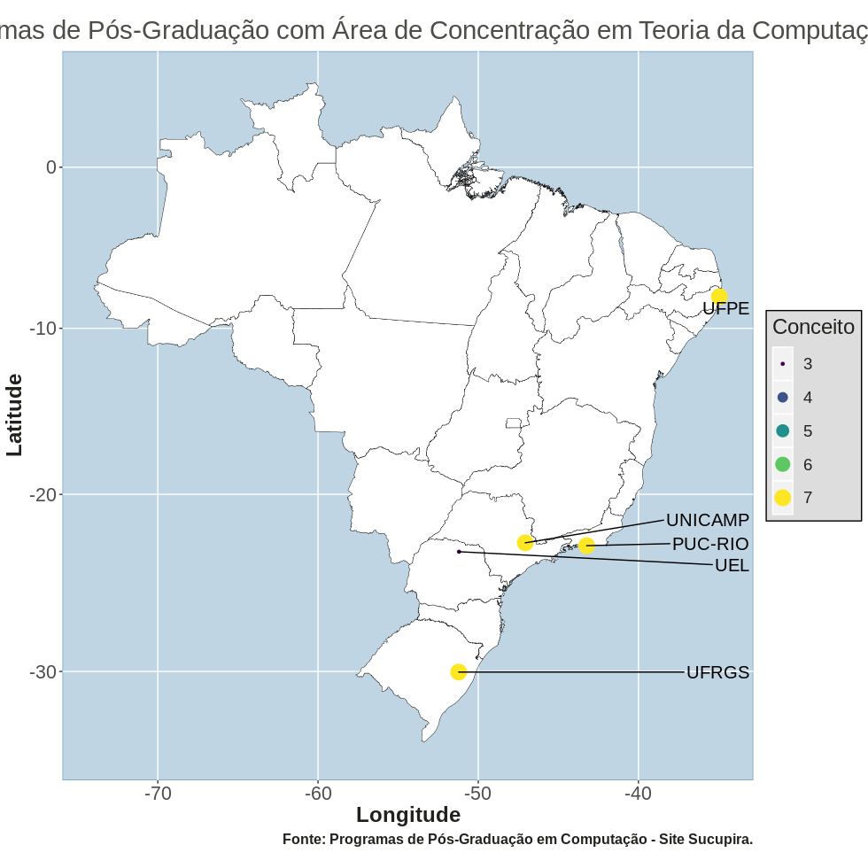
Brazilian Computer Graduating Programs that have Computer Theory as a concentration area.

all_data_2 <- subset(all_data, all_data$concentration_area == "Teoria da Computação")

ggplot() + 
geom_polygon(data = shape_brazil, aes(x = long, y = lat, group = group), fill = "white", size = 0.15, color = "black") +
geom_point(data = all_data_2[!duplicated(all_data_2$id),], aes(x = longitude, y = latitude, size = grade, color = grade)) +
geom_text_repel(data = all_data_2[!duplicated(all_data_2$code),], aes(x = longitude, y = latitude, label = code, size = 6), hjust = 0, nudge_x = -34 - subset(all_data_2, !duplicated(all_data_2$code))$longitude, direction = "y", show.legend = FALSE) +
scale_color_viridis(name = "Conceito", breaks = mybreaks) +
scale_size_continuous(name = "Conceito", breaks = mybreaks) +
coord_map() + 
guides(colour = guide_legend(), alpha = FALSE) +
ggtitle("Programas de Pós-Graduação com Área de Concentração em Teoria da Computação") +
labs + theme

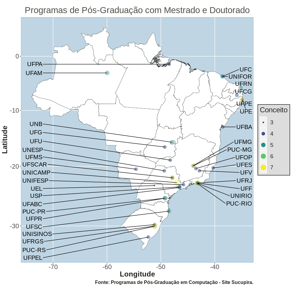
Brazilian Computer Graduating Programs that have both Master and Doctoral programs.

all_data_2 <- subset(all_data, all_data$graduation_level == "Mestrado e Doutorado Acadêmicos")

ggplot() + 
geom_polygon(data = shape_brazil, aes(x = long, y = lat, group = group), fill = "white", color = "black", size = 0.15) +
geom_point(data = all_data_2[!duplicated(all_data_2$id),], aes(x = longitude, y = latitude, size = grade, color = grade, shape = 19, alpha = I(2/grade))) +
geom_text_repel(data = all_data_2[all_data_2$longitude > -45 & !duplicated(all_data_2$code),], aes(x = longitude, y = latitude, label = code, size = 6), hjust = 0, nudge_x = -34 - subset(all_data_2, all_data_2$longitude > -45 & !duplicated(all_data_2$code))$longitude, direction = "y", show.legend = FALSE) +
geom_text_repel(data = all_data_2[all_data_2$longitude <= -45 & !duplicated(all_data_2$code),], aes(x = longitude, y = latitude, label = code, size = 6), hjust = 1, nudge_x = -72 - subset(all_data_2, all_data_2$longitude <= -45 & !duplicated(all_data_2$code))$longitude, direction = "y", show.legend = FALSE) + 
scale_shape_identity() +
scale_color_viridis(name = "Conceito", breaks = mybreaks) +
scale_size_continuous(name = "Conceito", breaks = mybreaks) +
coord_map() + 
guides(colour = guide_legend(), size = guide_legend()) +
ggtitle("Programas de Pós-Graduação com Mestrado e Doutorado") +
labs + theme

With the script below you can store this data into a database (postgresql in this example). Put your own postgres configuration below in password, dbname, host, port and user. Do not forget to create the tables, the full script is in SQL folder.

install.packages("RPostgreSQL")
require("RPostgreSQL")

password <- {
  "my_password"
}

drv <- dbDriver("PostgreSQL")
con <- dbConnect(drv, dbname = "my_database",
                 host = "localhost", port = 5432,
                 user = "my_user", password = password)
rm(pw) 

colnames(universities)[4] <- "course_id"
colnames(universities)[5] <- "level_id"

dbWriteTable(con, "university", value = universities, append = TRUE, row.names = FALSE)

colnames(research_names)[2] <- "name"
dbWriteTable(con, "research_topics", value = research_names, append = TRUE, row.names = FALSE)

dbWriteTable(con, "graduation_level", value = graduation_level, append = TRUE, row.names = FALSE)

colnames(brazilian_cities)[3] <- "latitude"
colnames(brazilian_cities)[4] <- "longitude"
dbWriteTable(con, "brazilian_cities", value = brazilian_cities, append = TRUE, row.names = FALSE)

dbWriteTable(con, "brazilian_states", value = brazilian_states, append = TRUE, row.names = FALSE)

dbWriteTable(con, "course_name", value = course_name, append = TRUE, row.names = FALSE)

dbWriteTable(con, "concentration_area", value = concentration_area, append = TRUE, row.names = FALSE)

colnames(university_research)[1] <- "id_university"
colnames(university_research)[2] <- "id_research_topics"
dbWriteTable(con, "university_research_topics", value = university_research, append = TRUE, row.names = FALSE)

colnames(university_concentration_area)[1] <- "id_university"
colnames(university_concentration_area)[2] <- "id_concentration_area"
dbWriteTable(con, "university_concentration_area", value = university_concentration_area, append = TRUE, row.names = FALSE)

dbDisconnect(con)
dbUnloadDriver(drv)

That's it. I need people to contribute with this project, to keep all this data up to date with Sucupira website. Anyone who wants to help, leave a message and let's work together.

jorgel-mendes/Graduating-Programs-Brazil

Summary

First Part

Second Part