Quality Complaints Classification

ML model to classify whether a quality complaint is valid or not. The model is trained on a fictional dataset of quality complaints and their corresponding labels.

Dataset

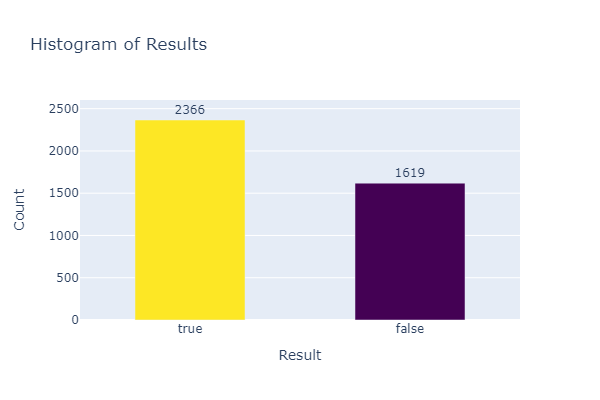
The fictional dataset consists of quality complaints and their corresponding results. The results are binary, where True indicates a valid complaint and False indicates an invalid complaint. The data columns are as follows:

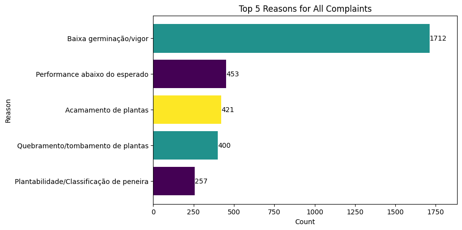
plant: The plant where the product was made
storage: The storage location of the product
quantity: The quantity of the product
number_defects: The number of defects in the product
sales: The volume of sales
location: The location of the complaint
hybrid: The hybrid (commercial name) of the product
treatment: The treatment of the product
reason: The reason for the complaint
result: The result of the complaint (True for valid, False for invalid)

Histograms

Statistical tests

Chi-Squared Test

The Chi-Squared Test of Independence is used to determine if there is a significant association between two categorical variables. The null hypothesis (H0) is that the variables are independent, and the alternative hypothesis (H1) is that the variables are dependent.

The formula is: $$\chi^2 = \sum \frac {(O - E)^2}{E}$$

Where $O$ is the observed frequency and $E$ is the expected frequency.

Cramer's V

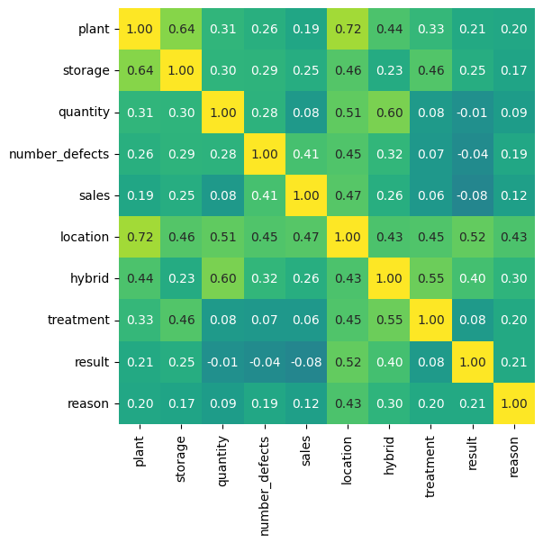
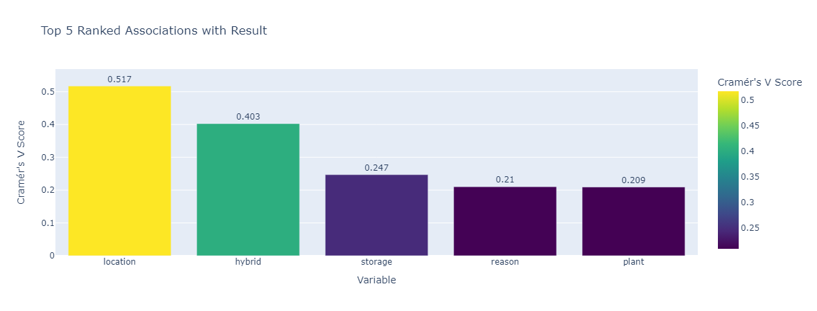
Cramer's V is a scaled version of the chi-squared test statistic $\chi^2$, which ranges from 0 to 1. It is used to measure the strength of association between two nominal variables. The value of Cramer's V ranges from 0 to 1, where 0 indicates no association between the variables, and 1 indicates a strong association between the variables.

The formula is: $$Cramer's V = \sqrt{\chi^2/(n\cdot(k-1))}$$

Where $\chi^2$ is the chi-squared test statistic, $n$ is the number of observations, and $k$ is the number of categories in the contingency table.

Models Development

The dataset is split into training and testing sets, with 80% of the data used for training and 20% for testing. The following models are trained on the dataset:

LightGBM
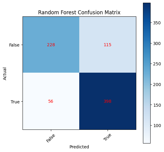
Random Forest

The models are evaluated using the following metrics:

Accuracy: The proportion of correct predictions to the total number of predictions.
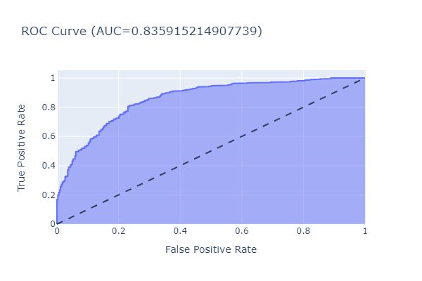
Roc-Auc: The area under the receiver operating characteristic curve, which measures the trade-off between true positive rate and false positive rate.

LightGBM

LightGBM is a gradient boosting framework that uses tree-based learning algorithms. It is designed for speed and efficiency and is widely used in machine learning competitions.

Random Forest

Random Forest is an ensemble learning method that constructs a multitude of decision trees during training and outputs the mode of the classes as the prediction.

Results

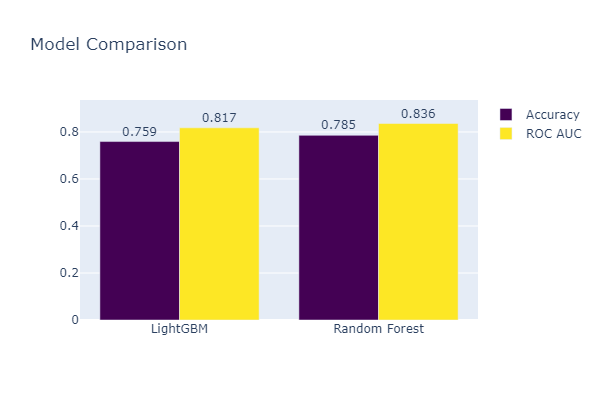
The results are as follows:

Model	Accuracy	Roc-Auc
LightGBM	0.759	0.817
Random Forest	0.785	0.836

The Random Forest model outperforms the LightGBM model in terms of accuracy and Roc-Auc score.

josehenriqueroveda/qc-classifier