Advanced Lane Finding Project
The goals / steps of this project are the following:
- Compute the camera calibration matrix and distortion coefficients given a set of chessboard images.
- Apply a distortion correction to raw images.
- Use color transforms, gradients, etc., to create a thresholded binary image.
- Apply a perspective transform to rectify binary image ("birds-eye view").
- Detect lane pixels and fit to find the lane boundary.
- Determine the curvature of the lane and vehicle position with respect to center.
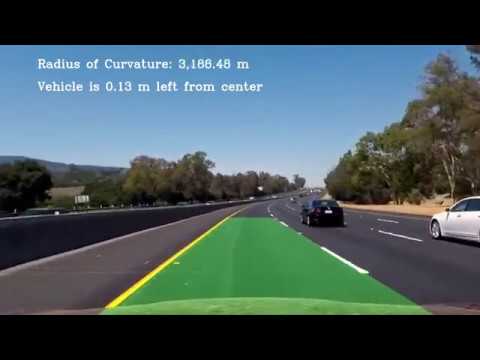
- Warp the detected lane boundaries back onto the original image.
- Output visual display of the lane boundaries and numerical estimation of lane curvature and vehicle position.
Rubric Points
Here I will consider the rubric points individually and describe how I addressed each point in my implementation.
You're reading it!
1. Briefly state how you computed the camera matrix and distortion coefficients. Provide an example of a distortion corrected calibration image.
The calibration does not need to be part of the video pipeline processing function, as the camera is the same for all frames. The calibration is thus calculated in a separate script called camera_calibration.py
I start by preparing "object points", which will be the (x, y, z) coordinates of the chessboard corners in the world. Here I am assuming the chessboard is fixed on the (x, y) plane at z=0, such that the object points are the same for each calibration image. Thus, objp is just a replicated array of coordinates, and objpoints will be appended with a copy of it every time I successfully detect all chessboard corners in a test image. imgpoints will be appended with the (x, y) pixel position of each of the corners in the image plane with each successful chessboard detection.
I then used the output objpoints and imgpoints to compute the camera calibration and distortion coefficients using the cv2.calibrateCamera() function. I applied this distortion correction to the test image using the cv2.undistort() function and obtained this result:


To demonstrate this step, I will show all the test images before and after applying distortion correction. The calibration is applied in pipeline.py, by the function cal_undistort() in lines 47 through 54


2. Describe how (and identify where in your code) you used color transforms, gradients or other methods to create a thresholded binary image. Provide an example of a binary image result.
Test5 image is the most difficult frame since it contains shadows and two different pavement colors. I used a script to test each gradient and hls color map separately, iterating through 25 possible values for each threshold. I chose each threshold individually and combined them using boolean logic to try to keep as much of the line as possible, while minimizing the background white pixels. (thresholding steps are part of the pipeline() method in pipeline.py lines 368 through 414). Here's the result of passing all the test images through the filters:


While some images may have some noise from shadow lines or hls inacuracies, I think this results will be good enough for the line detection.
3. Describe how (and identify where in your code) you performed a perspective transform and provide an example of a transformed image.
The code for my perspective transform includes a function called warp(), which appears in the file pipeline.py The warp() function takes as inputs an image (img), as well as the matrix calculated with cv2.getPerspectiveTransform and the src and destination dst points defined as follows:
Y_TOP = image_shape[1] * 0.64
Y_BOTTOM = image_shape[1]
TOP_W_HALF = 62
TOP_SHIFT = 4

roi_src = np.int32(
    [[(image_shape[0] * 0.5) - TOP_W_HALF + TOP_SHIFT, Y_TOP],
    [ (image_shape[0] * 0.16), Y_BOTTOM],
    [ (image_shape[0] * 0.88), Y_BOTTOM],
    [ (image_shape[0] * 0.5) + TOP_W_HALF + TOP_SHIFT, Y_TOP]])
roi_dst = np.int32(
    [[(image_shape[0] * 0.25), 0],
    [ (image_shape[0] * 0.25), image_shape[1]],
    [ (image_shape[0] * 0.75), image_shape[1]],
    [ (image_shape[0] * 0.75), 0]])
This resulted in the following source and destination points:
| Source | Destination |
|---|---|
| 583, 460 | 320, 0 |
| 230, 720 | 320, 720 |
| 1139, 720 | 960, 720 |
| 707, 460 | 960, 0 |
I verified that my perspective transform was working as expected by drawing the src and dst points onto a test image and its warped counterpart to verify that the lines appear parallel in the warped image.


4. Describe how (and identify where in your code) you identified lane-line pixels and fit their positions with a polynomial?
I implemented this step in lines 200 through 346s in my code in pipeline.py in the functions draw lane() and find_lane(). I used the polyfit math function to model the lane markers as a second order polynomial. A sliding window approach is used to identified the pixels that belong to lane markers. The sliding window is guided by the highest values in a histogram from the X-axis, which counts how many pixels where identified by the previous steps as being part of a clear line. Here are examples of my results on the test images:


5. Describe how (and identify where in your code) you calculated the radius of curvature of the lane and the position of the vehicle with respect to center.
To calculate the radius of curvature I used te technique suggested in class. The pixels that belong to the line are transformed to real world space by using a pixel to meter conversion factor. The coordinates in meters go into a polyfit math function to model each lane marker a second degree polynomial. The polynomial is then used to calculate the radius of curvature from the left and right lines. On the processed video the average curvature is displayed.
The distance to center is calculated based on the polynomial fit for the lines evaluated at the bottom of the image (y coordinate = 719). The center of the car is assumed to be at the 640th pixel. The center of the lane is the average x-coordinate of the two lanes at the bottom of the image. The distance is then converted from pixels to meters and displayed in the video.
The code to calculate the radius of curvature and distance from center is in the pipeline.py file, inside the find_lane() method, lines 270 to 288.
6. Provide an example image of your result plotted back down onto the road such that the lane area is identified clearly.
I implemented this step in lines 311 through 356 in my code in pipeline.py in the function draw_lane(). Here are examples of my results on the test images:


1. Provide a link to your final video output. Your pipeline should perform reasonably well on the entire project video (wobbly lines are ok but no catastrophic failures that would cause the car to drive off the road!).
Here's my final video:
1. Briefly discuss any problems / issues you faced in your implementation of this project. Where will your pipeline likely fail? What could you do to make it more robust?
My first approach did not include HLS color space threshold. This had a lot of problems when shadows from trees appear, but worked OK for an homogenious road. The H and S channels complement each other to overcome situations with shadows. In general I also had to readjust the settings multiple times as I progressed and realized my original threshold was not good enough after the next step.
The main pitfall my final implementation will find is that the Region of Interest used for the warp matrix definition is fixed. This assumes the car never leaves the lane, and will fail under a more curvy road than a highway.
Also, the light conditions for the project are really good (sunny day), this will fail under almost any other kind of lighting since the thresholds chosen are unflexible and they were calibrated only on sunny test images.
If I would pursue the project further I would widden the region of interest more. I would also store previous detections and use them as a prediction of where the next lanes can be expected. Reusing previous detections can help make the Region Of Interest more flexible, remove some "jumpiness" and discard false detections on more severe circumstances.