Python package for time-frequency analysis through Stockwell transform.
Based on original code from NIMH MEG Core Facility.
Part of this Python package is written in C, so you will need a C compiler.
On Linux (Debian or Ubuntu), install the build-essential package:
sudo apt install build-essential
On macOS, install the XCode Command Line Tools:
xcode-select --install
On Windows, install the Microsoft C++ Build Tools.
Make sure that you have FFTW installed.
If you use Anaconda (Linux, macOS, Windows):
conda install fftw
If you use Homebrew (macOS)
brew install fftw
If you use apt (Debian or Ubuntu)
sudo apt install libfftw3-dev
Finally, install this Python package using pip:
pip install .
Or, alternatively, in "editable" mode:
pip install -e .
Example usage:
import numpy as np
from scipy.signal import chirp
import matplotlib.pyplot as plt
from stockwell import st

t = np.linspace(0, 10, 5001)
w = chirp(t, f0=12.5, f1=2.5, t1=10, method='linear')

fmin = 0  # Hz
fmax = 25  # Hz
df = 1./(t[-1]-t[0])  # sampling step in frequency domain (Hz)
fmin_samples = int(fmin/df)
fmax_samples = int(fmax/df)
stock = st.st(w, fmin_samples, fmax_samples)
extent = (t[0], t[-1], fmin, fmax)

fig, ax = plt.subplots(2, 1, sharex=True)
ax[0].plot(t, w)
ax[0].set(ylabel='amplitude')
ax[1].imshow(np.abs(stock), origin='lower', extent=extent)
ax[1].axis('tight')
ax[1].set(xlabel='time (s)', ylabel='frequency (Hz)')
plt.show()
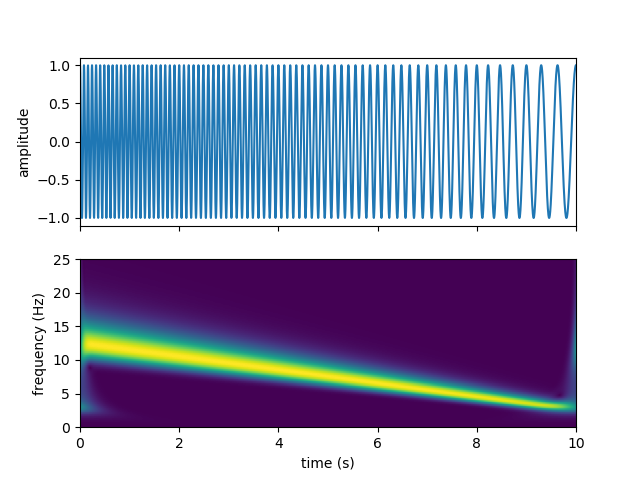
You should get the following output:
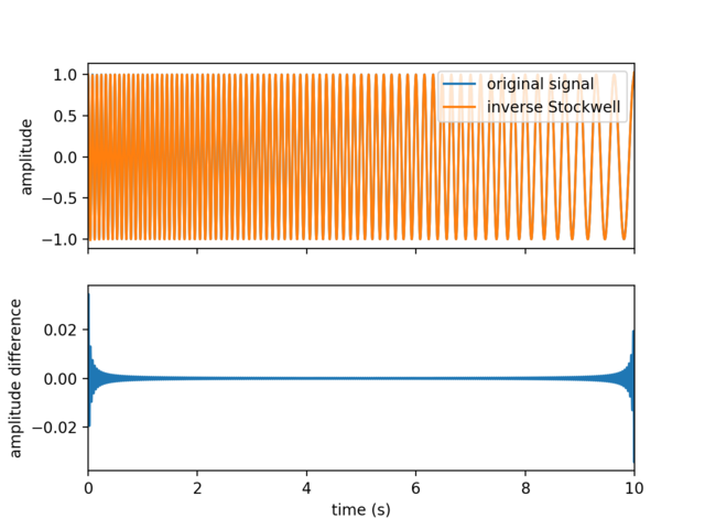
You can also compute the inverse Stockwell transform, ex:
inv_stock = st.ist(stock, fmin_samples, fmax_samples)
fig, ax = plt.subplots(2, 1, sharex=True)
ax[0].plot(t, w, label='original signal')
ax[0].plot(t, inv_stock, label='inverse Stockwell')
ax[0].set(ylabel='amplitude')
ax[0].legend(loc='upper right')
ax[1].plot(t, w - inv_stock)
ax[1].set_xlim(0, 10)
ax[1].set(xlabel='time (s)', ylabel='amplitude difference')
plt.show()Stockwell, R.G., Mansinha, L. & Lowe, R.P., 1996. Localization of the complex spectrum: the S transform, IEEE Trans. Signal Process., 44(4), 998–1001, doi:10.1109/78.492555

